Download
1 / 33
330 likes | 438 Views
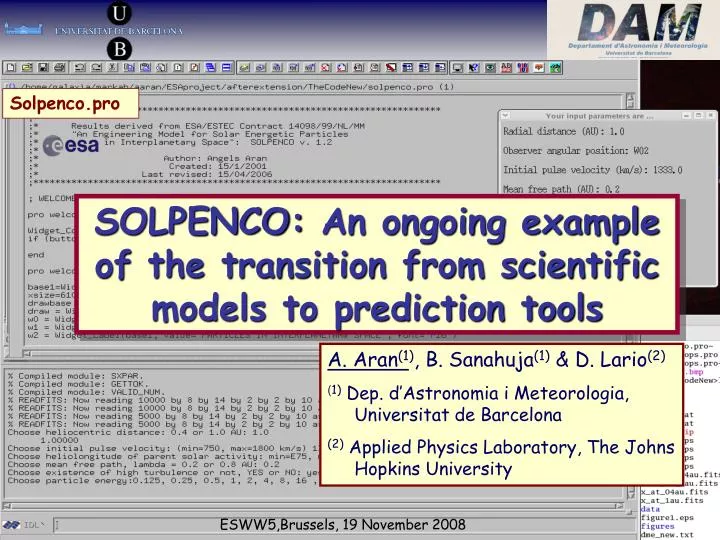
Solpenco.pro. SOLPENCO: An ongoing example of the transition from scientific models to prediction tools. A. Aran (1 ) , B. Sanahuja (1) & D. Lario (2) ( 1) Dep. d’Astronomia i Meteorologia, Universitat de Barcelona (2) Applied Physics Laboratory, The Johns Hopkins University.

E N D
Solpenco.pro SOLPENCO:An ongoing example of the transition from scientific models to prediction tools A. Aran(1), B. Sanahuja(1) & D. Lario(2) (1) Dep. d’Astronomia i Meteorologia, Universitat de Barcelona (2) Applied Physics Laboratory, The Johns Hopkins University ESWW5,Brussels, 19 November 2008
OUTLINE: • What is SOLPENCO? • How we built it up? • Fluxes & fluences of SEP events from SOLPENCO • Comparing the outputs with measurements • What must be improved? • Toward an improved version of SOLPENCO: SOLPENCO2 (within the SEPEM project)
What’s SOLPENCO? 4. Comparing with data • How is it built? 5. Improvements • Fluxes & Fluences 6. Toward SOLPENCO2 SOLPENCO (The SOLar Particle ENgineering COde) • Long-term objective: development of a tool to characterize SEP events at user-specified locations, from outside the solar corona up to the orbit of Mars. Main challenges: - knowledge of the underlying physics is incomplete - the scarce number of observations out of 1 AU. • SOLPENCO is a first step. Its main purpose is: To provide the capability to quantitatively and to rapidly predict SEP time-dependent upstream proton fluxes and fluences generated by interplanetary shocks, for 50 keV < E < ~100 MeV protons SOLPENCO allow us to analyze the aspects of SEP gradual events modeling that must be improved in order to produce useful space weather predictions.
What’s SOLPENCO? 4. Comparing with data • How is it built? 5. Improvements • Fluxes & Fluences 6. Toward SOLPENCO2 How does SOLPENCO work?
What’s SOLPENCO? 4. Comparing with data • How is it built? 5. Improvements • Fluxes & Fluences 6. Toward SOLPENCO2 Outputs of SOLPENCO. Examples Western event at 0.4 AU Central Meridian event at 1 AU Flux at 0.5 MeV Flux at 0.5 MeV Shock Shock Fluence E > 0.5 MeV Fluence E > 0.5 MeV
What’s SOLPENCO? 4. Comparing with data • How is it built? 5. Improvements • Fluxes & Fluences 6. Toward SOLPENCO2 The SOLPENCO tool SOLPENCO consists of: • A data base of pre-built SEP events • A user-friendly interface • A module that interpolates between the events in the database to obtain intermediate cases Note that: Modelling a given SEP event (e.g. with our Shock-and-Particle model, Lario et al., 1998) requires expertise and heavy computation (time). Thus, At present models cannot be directly applied for near-real time or rapid estimations of a given event eventually produced at the Sun.
What’s SOLPENCO? 4. Comparing with data • How is it built? 5. Improvements • Fluxes & Fluences 6. Toward SOLPENCO2 The database: brief description • Spacecraft Location a) Heliocentric distance, r:1 AU and 0.4 AU b)Angular position: from W90 to E75 (14 values) • Shock parameters: a) Initial pulse speed, vs: from 750 to 1800 km s-1 (8 values) b) Initial pulse width, : 140° (fixed) • Transport conditions: a) Proton mean free path (at 0.5 MeV), λ║: 0.2 AU and 0.8 AU. Scaled with proton rigidity λ║= λ║ (R/R0.5)2-q, q=1.5 b) Turbulent foreshock region: Yes/No option. (width = 0.1 AU; λ║c=0.01 AU (at 0.5 MeV); λ║c= λ║c (R/R0.5)-0.6 • Proton energies: from 0.125 to 64 MeV (10 values)
What’s SOLPENCO? 4. Comparing with data • How is it built? 5. Improvements • Fluxes & Fluences 6. Toward SOLPENCO2 Therefore, the data base contains: The flux and fluence computed for 10 energy channels, and 448 possibilities for the combined shock-particle scenario (8 shocks x 14 observers x 4 transport conditions) at 1 AU and at 0.4 AU. Taking into account the interpolated scenarios, SOLPENCO can provide the flux and fluence profiles for at least697,800 different events (Aran et al. 2006).
What’s SOLPENCO? 4. Comparing with data • How is it built? 5. Improvements • Fluxes & Fluences 6. Toward SOLPENCO2 The database: synthesising the flux profiles • We assume that the source of shock-accelerated particles Q is given by: • log Q (t, E) = log Q0(E) + k VR (t), • Based on the previous modelling of actual SEP events, • we adopted: • k = 0.5 • Q0 (E) = C Ewhere γ is the spectral index: γ = 2 for E < 2 MeV, and γ = 3 for E ≥ 2 MeV. γ -
By taking γ = 3 at high energy, we might be overestimating the fluence of a given event, in some cases. • What’s SOLPENCO? 4. Comparing with data • How is it built? 5. Improvements • Fluxes & Fluences 6. Toward SOLPENCO2 The database: A note on energy dependence At high energies the spectral index, γ, varies from 2 to 7 (Cane et al, 1998) This is a wide range!
2. First, the code interpolates between S/C locations for the same shock (upper plots) and then, it interpolates between the two initial speeds (bottom plot). • What’s SOLPENCO? 4. Comparing with data • How is it built? 5. Improvements • Fluxes & Fluences 6. Toward SOLPENCO2 Interpolation procedure Intermediate case 1200 km s-1 and W30 1. The code searches for both the initial speeds of the shock and s/c angular positions closest to the selection of the user
W001450W10 0.5 MeV • What’s SOLPENCO? 4. Comparing with data • How is it built? 5. Improvements • Fluxes & Fluences 6. Toward SOLPENCO2 Interpolation procedure Intermediate case obtained between correlative grid points: (1500 km s-1, W00) and (1350 km s-1, W00) Relative differences between simulated-interpolated events are less than a 10 %, except for the beginning of the event. Differences are much smaller.
What’s SOLPENCO? 4. Comparing with data • How is it built? 5. Improvements • Fluxes & Fluences 6. Toward SOLPENCO2 Flux profiles The difference between the profiles corresponding to the same initial shock speeds in the top and bottom panels is a direct consequence of the different conditions for the particle acceleration and injection in the regions scanned by the cobpoint.
What’s SOLPENCO? 4. Comparing with data • How is it built? 5. Improvements • Fluxes & Fluences 6. Toward SOLPENCO2 Observer’s location Shock strength Peak Fluxes The faster the shock the higher the peak flux, for the same angular position. At 1 AU, for each interplanetary shock, western central meridian events (W00-W15) have the higher peak fluxes.
What’s SOLPENCO? 4. Comparing with data • How is it built? 5. Improvements • Fluxes & Fluences 6. Toward SOLPENCO2 Observer’s location Shock strength Fluences • Two factors determine the fluence: (1) the duration of the injection of shock-accelerated particles and (2) the efficiency of the shock as a particle accelerator.
What’s SOLPENCO? 4. Comparing with data • How is it built? 5. Improvements • Fluxes & Fluences 6. SOLPENCO2 Fluences • A relevant result: the fluence derived for SEP events at 1 AU are higher than those obtained at 0.4 AU. This is against the inverse squared power law dependence of the fluence with the heliocentric distance, usually assumed. • This is a consequence of the contribution to the fluence of the interplanetary shock which is more important as longer the duration of the particle event is and stronger the shock is. But, the shock-and-particle model does not consider the contribution of the downstream region of the SEP events. In certain scenarios, this could lead to higher cumulate fluences than those predicted by the model.
What’s SOLPENCO? 4. Comparing with data • How is it built? 5. Improvements • Fluxes & Fluences 6. Toward SOLPENCO2 W00, 1AU IMF E30,0.4 AU Radial dependences Let’s assume for a pair of observers that: F(0.4)/F(1.0) = 0.4β where F is the fluence or the peak intensity and β is the radial index PEAK INTENSITIES
What’s SOLPENCO? 4. Comparing with data • How is it built? 5. Improvements • Fluxes & Fluences 6. Toward SOLPENCO2 Radial dependences Even for observers located along the same IMF line the radial dependence of the peak flux depends on: (1) the longitudinal separation between the spacecraft’s and the direction toward the shock expands and (2) the shock front region along which the observer is connected (i.e. the regions scanned by the cobpoint). For well-connected events: The higher the shock speed, the fastest the decrease of the peak flux with the heliocentric distance. Event fluences are calculated here up to the arrival of the shock. Their radial dependence are positive because the duration of the SEP events is longer at 1 AU than at 0.4 AU.
What’s SOLPENCO? 4.Comparing with data • How is it built? 5. Improvements • Fluxes & Fluences 6. SOLPENCO2 Comparison with observations Selection of the SEP events We identified the solar origin of 115 interplanetary shocks associated with proton events (SEP events) between January 1998 and October 2001. We used observations of ten (47 keV < E < 440 MeV) channels from ACE/EPAM and IMP8/CPME instruments. • Selection criteria: SEP events for which • The association between the shock and a parent solar activity is well established and unique • The proton intensity-time profiles show a significant increase of the flux profiles for E < 25 MeV and there is a noticeable enhancement up to 96 MeV • The SEP event is not superimposed on a preceding event.
What’s SOLPENCO? 4.Comparing with data • How is it built? 5. Improvements • Fluxes & Fluences 6. Toward SOLPENCO2 Comparison with observations The output is a set of 16 SEP events: 8 Central meridian events (E30 – W30) and
What’s SOLPENCO? 4.Comparing with data • How is it built? 5. Improvements • Fluxes & Fluences 6. Toward SOLPENCO2 7 Western events (W30 – >W90) and 1 Eastern event Western events
What’s SOLPENCO? 4.Comparing with data • How is it built? 5. Improvements • Fluxes & Fluences 6. Toward SOLPENCO2 Flux at shock arrival Peak flux Analysis of the peak intensities An example: 12 – 15 Sep 2000, W09 SEP event Example of a central meridian event
What’s SOLPENCO? 4.Comparing with data • How is it built? 5. Improvements • Fluxes & Fluences 6. Toward SOLPENCO2 Analysis of the peak intensities
What’s SOLPENCO? 4.Comparing with data • How is it built? 5. Improvements • Fluxes & Fluences 6. Toward SOLPENCO2 Analysis of the peak intensities The peak fluxes of the analyzed central meridian (western) SEP events are well predicted at E < 2 MeV. Predictions of central meridian events are still valid at high energies for the events with a relatively poor contribution of a particle population accelerated when the shock is still close to the Sun. For events displaying a strong prompt component predictions do not match observations at E > 2 MeV. • The reason is twofold: • The initial conditions of the MHD code are placed at 18R, thus above the region where the injection of the high-energy particles is assumed to take place; and • the constant of proportionality between Q and VR (k = 0.5) has been derived from modeling actual SEP events at low energies.
What’s SOLPENCO? 4. Comparing withdata • How is it built? 5. Improvements • Fluxes & Fluences 6. SOLPENCO2 What must be improved? • Main (internal) difficulties when building SOLPENCO: • ● The slope k in Q(VR) • ● The spectral index, γ Main (external) shortcomings: ●MHD modeling and initial conditions ●Proxy solar indicators/conditions (type II, CME speed,…) ●Lack of observational data out of 1 AU (i.e., 0.3 AU and 1.5 AU) to study radial gradients ( a lot of work to do!)
What’s SOLPENCO? 4. Comparing withdata • How is it built? 5. Improvements • Fluxes & Fluences 6. Toward SOLPENCO2 What would happen if the cobpoint could be tracked closer to the Sun? Improving the code An example western event of 2 October 1998 MeV The conclusion: A MHD shock propagation model with an inner boundary near 3-4 R would represent a large improvement of the present version of SOLPENCO. Shock Contribution of shock-accelerated particles to the flux during the prompt phase of the event
What’s SOLPENCO? 4. Comparing withdata • How is it built? 5. Improvements • Fluxes & Fluences 6. Toward SOLPENCO2 Improving the code An example of a CME-driven shock simulation: Observer at W60 • We are collaborating with the group in the Center for Plasma Astrophysics (CPA), Leuven (Belgium). • They have a 2D MHD model to simulate the propagation of CME-driven shocks from the inner corona to 1.7 AU. • Its initial boundary at ~3 R will allow us to track the initial stages of SEP events where the acceleration of particles in more efficient. MHD simulation by Carla Jacobs (CPA, K.U.Leuven)
What’s SOLPENCO? 4. Comparing withdata • How is it built? 5. Improvements • Fluxes & Fluences 6. Toward SOLPENCO2 Changing the shock-and-particle model The April 2000 SEP event: an example MHD simulation by Carla Jacobs (CPA, K.U.Leuven)
What’s SOLPENCO? 4. Comparing withdata • How is it built? 5. Improvements • Fluxes & Fluences 6. Toward SOLPENCO2 Changing the shock-and-particle model Fitting plasma parameters at 1 AU: ACE/MAG and SWEPAM data Simulation MHD simulation by Carla Jacobs (CPA, K.U.Leuven)
What’s SOLPENCO? 4. Comparing withdata • How is it built? 5. Improvements • Fluxes & Fluences 6. Toward SOLPENCO2 Changing the shock-and-particle model Position of the COBPOINT The magnetic connection of the observer with the shock front is established at: time r-distance Run1 0.17 h 4.3 R Run2 0.33 h 5.3 R MHD old 1 3.4 h 25.5 R MHD old 2 3.5 h 25.0 R VR (t) Source of shock-accelerated particles Q is given by: log Q (t, E) = log Q0(E) + k VR (t)
What’s SOLPENCO? 4. Comparing withdata • How is it built? 5. Improvements • Fluxes & Fluences 6. Toward SOLPENCO2 Changing the shock-and-particle model Fitting particle fluxes at 1 AU ACE/EPAM data Simulation The only assumed source of particles is the coronal/IP CME-driven shock.
What’s SOLPENCO? 4. Comparing withdata • How is it built? 5. Improvements • Fluxes & Fluences 6. Toward SOLPENCO2 Conclusion: Toward SOLPENCO2 • We are working to produce an improved shock-and-particle model to built a new particle flux and fluence data base for SOLPENCO SOLPENCO2 • This is part of the SolarEnergetic Particle Environment Modelling (SEPEM)Projectsponsored by ESA in which we (STP/SW Group/CPA) are involved. • SOLPENCO2 must provide rapid and improved synthetic particle flux profiles for observers located from ~0.1 AU up to 1.7 AU and covering a wider range of heliolongitudes. See the poster by P.T.A Jiggens et al. “The ESA SEPEM Project: Database and Tools”
“The two extremes” Prediction • What’s SOLPENCO? 4. Comparing with data • How is it buit? 5. Improvements • Fluxes & Fluences 6. SOLPENCO2 THANKS!! three