Information Theory

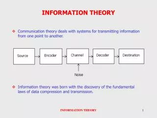
1. Information Theory Recommended readings: Simon Haykin: Neural Networks: a comprehensive foundation, Prentice Hall, 1999, chapter “Information Theoretic Models”. Hyvärinen, J. Karhunen, E. Oja: Independent Component Analysis Wiley, 2001. What is the goal of sensory coding? Attneave (1954): “A major function of the perceptual machinery is to strip away some of the redundancy of stimulation, to describe or encode information in a form more economical than that in which it impinges on the receptors.”

2. Motivation Observation: Brain needs representations that allow efficient access to information and do not waste precious resources. We want efficient representation and communication. A natural framework for dealing with efficient coding of information is information theory, which is based on probability theory. Idea:the brain may employ principles from information theory to code sensory information from the environment efficiently.

3. Dayan and Abbott Observation: (Baddeley, 1997) Neurons in lower (V1) and higher (IT) visual cortical areas, show approximately exponential distribution of firing rates in response to natural video (panel A). Why may this be?

4. What is the goal of sensory coding? • Sparse vs. compact codes: • two extremes: PCA (compact) vs. Vector Quantization • Advantages of sparse codes (Field, 1994): • signal-to-noise ratio: • small set of very active units above “sea of inactivity” • correspondence and feature detection: • small number of active units facilitates finding the right • correspondences, higher order correlations are rarer and thus more • meaningful • storage and retrieval with associative memory: • storage capacity greater in sparse networks (e.g. Hopfield)

5. What is the goal of sensory coding? Another answer: Find independent causes of sensory input. Example: image of a face on the retina depends on identity, pose, location, facial expression, lighting situation, etc. We can assume that these causes are close to independent. Would be nice to have a representation that allows easy read out of (some of) the individual causes. Example: Independence: p(a,b)=p(a)p(b) p(identity, expression)=p(identity)p(expression) (factorial code)

6. What is the goal of sensory coding? • More answers: • Fish out information relevant for survival (markings of prey and • predators). • Fish out information that lead to rewards and punishments. • Find a code that allows good generalizations. Situations requiring • similar actions should have similar representations • Find representations that allow different modalities to talk to • one another, facilitate sensory integration. • Information theory gives us a mathematical framework for discussing some but not all of these issues. Only speaks about probabilities of • symbols/events but not their meaning.

7. Efficient coding and compression • Saving space on your computer hard disk: • use “zip” program to compress files, store images and movies • in “jpg” and “mpg” formats • lossy versus loss-less compression • Example: Retina • When viewing natural scenes, the firing of neighboring rods or • cones will be highly correlated. • Retina input: ~108 rods and cones • Retina output: ~106 fibers in optic nerve, reduction by factor ~100 • Apparently, visual input is efficiently re-coded to save resources. • Caveat: Information theory just talks about symbols, messages • and their probabilities but not their meaning, e.g., how • survival relevant they are for the organism.

8. Communication over noisy channels Information theory also provides a framework for studying information transmission across noisy channels where messages may get compromised due to noise. Examples: modem → phone line → modem Galileo satellite → radio waves → earth daughter cell parent cell daughter cell computer memory → disk drive → computer memory

9. Recall: Matlab: LOG, LOG2, LOG10 Note: base of logarithm is matter of convention, in information theory base 2 is typically used: information measured in bits in contrast to nats for base e(natural logarithm).

10. How to Quantify Information? consider discrete random variable X taking values from the set of “outcomes” {xk, k=1,…,N} with probability Pk: 0≤Pk≤1; ΣPk=1 Question: what would be a good measure for the information gained by observing outcome X= xk ? Idea: Improbable outcomes should somehow provide more information Let’s try: “Shannon information content” Properties: I(xk) ≥ 0 since 0≤Pk≤1 I(xk) = 0 for Pk=1 (certain event gives no information) I(xk) > I(xi) for Pk < Pi logarithm is monotonic, i.e: if a<b then log(a)<log(b)

11. Information gained for sequenceof independent events Consider observing the outcomes xa, xb, xc in succession; the probability for observing this sequence is P(xa,xb,xc) = PaPbPc Let’s look at the information gained: I(xa,xb,xc) = - log(P(xa,xb,xc)) = -log(PaPbPc) = -log(Pa)-log(Pb)-log(Pc) Information gained is just the sum of individual information gains = I(xa) + I(xb) +I(xc)

12. Entropy Question: What is the average information gained when observing a random variable over and over again? Answer: Entropy! • Notes: • entropy always bigger than or equal to zero • entropy is a measure of the uncertainty in a random variable • can be seen as generalization of variance • entropy related to minimum average code length for variable • related concept in physics and physical chemistry: there entropy is a measure of the “disorder” of a system.

13. Answer: (just apply definition) Examples 1. Binary random variable: outcomes are {0,1} where outcome ‘1’ occurs with probability P and outcome ‘0’ occurs with probability Q=1-P. Question: What is the entropy of this random variable? Note: entropy zero if one outcome certain, entropy maximized if both outcomes equally likely (1 bit)

14. 2. Horse Race: eight horses are starting and their respective odds of winning are: 1/2, 1/4, 1/8, 1/16, 1/64, 1/64, 1/64, 1/64 What is the entropy? H = -(1/2 log(1/2) + 1/4 log(1/4) + 1/8 log(1/8) + 1/16 log(1/16) + 4 * 1/64 log(1/64) = 2 bits What if each horse had chance of 1/8 of winning? H = -8 * 1/8 log(1/8) = 3 bits (maximum uncertainty) 3. Uniform: for N outcomes entropy maximized if all equally likely:

15. Entropy and Data Compression Note: Entropy is roughly the minimum average code length required for coding a random variable. Idea: use short codes for likely outcomes and long codes for rare ones. Try to use every symbol of your alphabet equally often on average (e.g. Huffman coding described in Ballard book). This is basis for data compression methods. Example: consider horse race again: Probabilities of winning: 1/2, 1/4, 1/8, 1/16, 1/64, 1/64, 1/64, 1/64 Naïve code: 3 bit combination to indicate winner: 000, 001, …, 111 Better code: 0, 10, 110, 1110, 111100, 111101, 111110, 111111 requires on average just 2 bits (the entropy), 33% savings !

16. Differential Entropy • Idea: generalize to continuous random variables described by pdf: • Notes: • differential entropy can be negative, in contrast to entropy of discrete random variable • but still: the smaller differential entropy, the “less random” is X • Example: uniform distribution

17. Maximum Entropy Distributions Idea: maximum entropy distributions are “most random” For discrete RV, uniform distribution has maximum entropy For continuous RV, need to consider additional constraints on the distributions: Neurons at very different ends of the visual system show the same exponential distribution of firing rates in response to “video watching” (Baddeley et al., 1997)

18. Why exponential distribution? Exponential distribution maximizes entropy under the constraint of a fixed mean firing rate µ. Maximum entropy principle: find density p(x) with maximum entropy that satisfies certain constraints, formulated as expectations of functions of x: Answer: Interpretation of mean firing rate constraint: each spike incurs certain metabolic costs: goal is to maximize transmitted information given a fixed average energy expenditure

19. Examples • Two important results: • for a fixed variance, the Gaussian distribution has the highest entropy (another reason why the Gaussian is so special) • for a fixed mean and p(x)=0 if x≤0, the exponential distribution has the highest entropy. Neurons in brain may have exponential firing rate distributions because this allows them to be most “informative” given a fixed average firing rate, which corresponds to a certain level of average energy consumption

20. Intrinsic Plasticity • Not only the synapses are plastic! Now surge of evidence for adaptation of dendritic and somatic excitability. Typically associated with homeostasis ideas, e.g.: • neuron tries to keep mean firing rate at desired level • neuron keeps variance of firing rate at desired level • neuron tries to attain particular distribution of firing rates

21. Question: how do intrinsic conductance properties need to change to reach specific firing rate distribution? Stemmler&Koch (1999): derived learning rule for two compartment Hodgkin-Huxley model: where gi is the (peak) value of the i-th conductance adaptation of gi leads to learning... … of uniform firing rate distribution Question 1: formulations of intrinsic plasticity for firing rate models? Question 2: how do intrinsic and synaptic learning processes interact?

22. Pk Qk 1 2 3 4 5 6 1 2 3 4 5 6 Kullback Leibler Divergence Idea: Consider you want to compare two probability distributions P and Q that are definedover the same set of outcomes. unfair dice A “natural” way of defining a “distance” between two distributions is the so-called Kullback-Leibler divergence (KL-distance), or relative entropy:

23. Properties of KL-divergence: D(P||Q) ≥ 0 and D(P||Q)=0 if and only if P=Q, i.e., if two distributions are the same, their KL-divergence is zero otherwise it’s bigger. D(P||Q) in general is not equal to D(Q||P) (i.e. D(.||.) is not a metric) The KL-divergence is a quantitative measure of how “alike” two probability distributions are. Generalization to continuous distributions: The same properties as above hold.

24. Mutual Information Consider two random variables X and Y with a joint probability mass function P(x,y), and marginal probability mass functions P(x) and P(y). Goal: KL-divergence is quantitative measure of “alikeness” of distributions of two random variables. Can we find a quantitative measure of independence of two random variables? Idea: recall definition of independence of two random variables X,Y: We define as the mutual information the KL-divergence between the joint distribution and the product of the marginal distributions:

25. Properties of Mutual Information: • I(X;Y)≥0, equality if and only if X and Y are independent • I(X;Y) = I(Y;X) (symmetry) • I(X;X) = H(X), entropy is “self-information” Generalization to multiple RVs: deviation from independence savings in encoding

26. Mutual Information as Objective Function Haykin Linsker’s Infomax ICA Imax by Becker and Hinton Note: trying to maximize or minimize MI in a neural network architecture sometimes leads to biologically implausible non-local learning rules

27. Cocktail Party Problem Motivation: cocktail party with many speakers as sound sources and array of microphones, where each microphone is picking up a different mixture of the speakers. Question: can you “tease apart” the individual speakersjust given x, i.e. without knowing how the speakers’ signals got mixed? (Blind source separation (BSS))

28. Blind Source Separation Example original time series of source s linear mixture x unmixed signals: Demos of blind audio source separation: http://www.cnl.salk.edu/~tewon/Blind/blind_audio.html

29. Definition of ICA • Note: there are several, this is the simplest and most restrictive: • sources are independent and non-gaussian: s1, …, sn • sources have zero mean • n observations are linear mixtures: • the inverse of A exists: • Goal: find this inverse. Sine we do not know the original, can cannot compute it directly but we will have to estimate it: • once we have our estimate, we can compute the sources: • Relation of BSS and ICA: • ICA is one method of addressing BSS, but not the only one • BSS is not the only problem where ICA can be usefully applied

30. Restrictions of ICA • Need to require: (it’s surprisingly little we have to require!) • sources are independent • sources are non-gaussian (at most one can be gaussian) • Ambiguities of solution: • sources can be estimated only up to a constant scale factor • may get permutation of the sources, i.e. sources may not be recovered in their right order a) multiplying source with constant and dividing that source’s matrix entries by same constant leaves x unchanged b) switching these columns leaves x unchanged

31. Projection Pursuit: find projection along which data looks most “interesting” Projection Pursuit PCA Principles for Estimating W: • Several possible objectives (contrast functions): • requiring outputs yi to be uncorrelated is not sufficient • outputs yi should be maximally independent • outputs yi should be maximally non-gaussian, • (central limit theorem), (projection pursuit) • maximum likelihood estimation • Algorithms: • various different algorithms based on • these different objectives with interesting • relationships between them • to evaluate criteria like independence (MI), need to • make approximations since distributions unknown • typically, whitening is used as a • pre-processing stage (reduces number • of parameters that need to be estimated)

32. Artifact Removal in MEG Data original MEG data ICs found with ICA algorithm

33. ICA on Natural Image Patches • The basic idea: • consider 16 by 16 gray scale patches of natural scenes • what are the “independent sources” of these patches? • Result: • they look similar to V1 simple cells: localized, oriented, bandpass • Hypothesis: • Finding ICs may be principle of sensory coding in cortex! • Extensions: • stereo/color images, non-linear methods, topographic ICA

34. Discussion: Information Theory • Several uses: • Information theory is important for understanding sensory coding and information transmission in nervous systems • Information theory is a starting point for developing new machine learning and signal processing techniques such as ICA • Such techniques can in turn be useful for analyzing neuroscience data as seen in the EEG example • Caveat: • Typically difficult to derive biologically plausible learning rules from information theoretic principles. Beware of non-local learning rules.

35. Some other limitations The “standard approach” for understanding visual representations: The visual system tries to find efficient encoding of random natural image patches or video fragments that optimizes statistical criterion: sparseness, independence, temporal continuity or slowness Is this enough for understanding higher level visual representations? Argument 1:the visual cortex doesn’t get to see random image patches but actively shapes the statistics of its inputs Argument 2:approaches based on trace rules break down for discontinuous shifts caused by saccades Argument 3:vision has to serve action: the brain may be more interested in representations that allow efficient acting, predict rewards etc. Yarbus (1950s): vision is active and goal-directed

36. Building Embodied Computational Models of Learning in the Visual System • Anthropomorphic robot head: • 9 degrees of freedom, dual 640x480 color images at 30 Hz • Autonomous Learning: • unsupervised learning, reinforcement learning (active), innate biases

37. Simple illustration: clustering of image patches an “infant vision system” looked at b: system learning from random image patches c: system learning from “interesting” image patches (motion, color) The biases, preferences, and goals of the developing system may be as important as the learning mechanism itself: the standard approach needs to be augmented!