Download
1 / 36
360 likes | 508 Views
Off-Axis Telescopes for Dark Energy Investigations. SPIE 7731-52, 30 June 2010 M.Lampton (UC Berkeley) M. Sholl (UC Berkeley) M. Levi (LBNL Berkeley). Dark Energy?. A name we give to describe the observed acceleration of the expansion of the universe

E N D
Off-Axis Telescopes for Dark Energy Investigations SPIE 7731-52, 30 June 2010 M.Lampton (UC Berkeley) M. Sholl (UC Berkeley) M. Levi (LBNL Berkeley)
Dark Energy? • A name we give to describe the observed acceleration of the expansion of the universe • Could be the “cosmological constant” in GR • Very hard to explain why that isn’t huge, or zero • Could be something else! • Varying over time; maybe even over space! • Different theories predict how DE evolves • Test: BAO – a standard ruler, shows expansion history • Test: SNe – a standard candle, shows expansion history • Test: WL – shows growth of structure over history Lampton Sholl & Levi 2010
Baryon Acoustic Oscillations: standard rulers http://mwhite.berkeley.edu/BAO/bao_iucca.pdf How to measure redshifts of 30 million galaxies per year, with σz = 0.001/(1+z)? Use slitless spectroscopy! Komatsu et al arXiv 1001.4538 Then: z=1100 Ruler = 400kly Now: z=0 Ruler = 400Mly Tighter PSF => smaller σz => Bigger Survey Lampton Sholl & Levi 2010
Type Ia Supernovae: standard candles Red: SNR at peak. Others: earlier and later times Kowalski et al., ApJ 686, 749 (2008) Peak spectrum Reference spectrum explosion Figures courtesy A.G.Kim 2010 Tighter PSF => Less Texp > Bigger Survey Lampton Sholl & Levi 2010
Weak Lensing: probe growth of structure Space based WL program seeks 30 galaxies/sqarcmin, 0.2 arcsec, 25th mag galaxies; needs good PSF and stability Strong lensing A2218 http://www.cita.utoronto.ca/~hoekstra/lensing.html Weak lensing statistical concept Rhalf, arcseconds Jouvel et al., “Designing Future Dark Energy Missions” A&A 504, 359 (2009) Tight PSF and small pixels are mandatory to get these galaxies Lampton Sholl & Levi 2010
JDEMInterim Science Working Group Report http://jdem.lbl.gov (2010) Lampton Sholl & Levi 2010
JDEMInterim Science Working Group Report http://jdem.lbl.gov (2010) Lampton Sholl & Levi 2010
Key Mission Requirement: Survey Rate • Simple formulas like… • JSIM: a public web tool created by M.Levi • http://jdem.lbl.gov/ “Exposure Time Calculator” • JSIM inputs are high-level mission parameters • Telescope Aperture, central obstruction size, WFE… • Field of view on sky, pixel scale, focal length, number of sensor chips • Detector Technology: pixel size, pixels per chip, waveband, QE curve • Fraction of time allocated to BAO, SNe, WL, calibration, downlink, … • Mission duration • JSIM outputs are “high level” mission yield & FOMs • JSIM outputs also available at “low level” individual FO’s. • Bottom line: smaller point spread function boosts yields This talk Lampton Sholl & Levi 2010
JSIM Internal Databases & Models http://jdem.lbl.gov/ “Exposure Time Calculator” • BAO emission line galaxy Hα flux, size, and redshift distribution • Ilbert et al 2005 • WL galaxy magnitude, size, and redshift distribution • Leauthaud et al 2008 zCOSMOS; Jouvel et al 2009 • Supernova occurrence rate vs redshift • Lesser of published curves by Sullivan et al 2006 and Dahlen et al 2008 • Zodiacal light vs wavelength and ecliptic latitude • Leinert et al 1998; Aldering 2001 • Optical point spread function • MTF contributions from pupil diffraction and WFE via Fischer’s Hopkins Ratio • Gaussian two dimensional random attitude control errors • Sensor pixel size; interpixel diffusion • Sensor contributions (dark current, read noise, QE) • Signal-to-noise ratio estimation • Optimal extraction, convolving galaxy exponential with system PSF Lampton Sholl & Levi 2010
Obscured vs Unobscured Focal TMAsThese historical examples are both focal but afocal configurations are equally good Obscured, here with 1.2m aperture f/11; 13mEFL 18um = 0.285” FoV = 0.73x1.46deg =166 x 330mm Easy fit to 4x8 sensors. < 3umRMS theoretical PSF Real Cassegrain image: control stray light Real exit pupil: control of stray heat Best with auxiliary optics behind PM; Easy heat path for one focal plane. Korsch,D., A.O. 16 #8, 2074 (1977) Unobscured, also with 1.2m aperture f/11, 13mEFL, 18um=0.285” FOV = 0.73 x1.46deg = 166x330mm Easy fit to 4x8 sensors. < 3umRMS theoretical PSF Real Cassegrain image: control stray light Real exit pupil: control of stray heat Easy heat path to cold side of payload for entire SM-TM-FP assembly; can accommodate several focal planes. Cook,L.G., Proc.SPIE v.183 (1979) Lampton Sholl & Levi 2010
PSFs For Unaberrated Pupils Scaled for equal incident flux and equal PM diameter Shows both obstructed light loss and diffraction loss Fresnel-Kirchoff diffraction integral Unobstructed Obstructed: 50% linear, 25% area Lampton Sholl & Levi 2010
Encircled Energy as a Fraction of the Total Transmitted Light with no aberrations Fresnel-Kirchoff diffraction integral: Schroeder 10.2 Linear obstruction = 0%, 10%, 20%, 30%, 40%, 50% Lampton Sholl & Levi 2010
EE50 Radius (arcsec) ComparisonHeld constant: f/11, WFE=0.1µm rms, pixel =18µm, blur= 1µm, ACS blur=0.02 arcsec. • Results show little difference in the visible since we are not diffraction limited there • However longward of one micron, diffraction dominates the PSF, and the unobscured looks attractive. • On the faintest targets, Rhalf hurts you like its square (ouch) 1.1m obscured 1.3m obscured 1.1m unobscured 1.3m unobscured Wavelength microns Lampton Sholl & Levi 2010
Eliminating the SM support spider legs HST file image courtesy STScI At Galactic midlatitudes, diffraction rings and spikes bring the focal plane irradiance to twice Zodi over 1% of random locations. Elimination: slightly improved survey efficiency; eases background subtraction, reduced “coverage gap” correlation . Lampton Sholl & Levi 2010
Some Unobscured Concepts Lampton Sholl & Levi 2010
Manufacturing & Testing Challenges? • Off-axis: more material removal and greater aspheric departure • Off-axis: non axisymmetric test setups need more time & care • Existence proof: Giant Magellan Telescope segments: 8.4m! • Today’s laser trackers can deliver submicron surface metrology • Vendors caution us that going off-axis is do-able but not “free” Lampton Sholl & Levi 2010
Payload Packaging Challenges? • Traditional space telescope payloads are on-axis cylinders • Traditionally the launch fairing is a cylinder plus an ogive extension • Good match! • Off-axis telescope is not a good match • However … going to Earth-Sun L2 Lagrange point requires an EELV whose launch fairing is 4m diameter. Plenty of room for any layout of a 1.1 m aperture telescope • As presently envisioned, JDEM packaging is not constrained by EELV fairing, even though off axis Lampton Sholl & Levi 2010
Many JDEM Trade Studies RemainContent et al.; Sholl et al.; Lieber et al.; Noecker; Edelstein et al.; Besuner et al.; Reil et al. • Focal vs Afocal rear-end architecture • Imager requirements and design • Field of view; plate scale; pixel size; waveband(s)… • How to calibrate it: flats, darks, wavelength, linearity… • Wide field spectrometer requirements • Field of view; plate scale; pixel size; waveband… • Resolving power; issue of redshift accuracy. • How to calibrate it: flats, darks, wavelength, linearity… • Supernova spectrometer requirements • Single slit vs integral field slicer architecture • Field of view; plate scale; pixel size; waveband • How to calibrate it: flats, darks, wavelength, linearity… • The overall mission design: how to best integrate objectives • And then… of course … there’s all the engineering! Lampton Sholl & Levi 2010
Obscured Unobscured • Traditional in space astronomy • Axisymmetric PM has lower manufacture & test cost for given aperture because total departure from sphere is less • If Wide field: SM baffle is large then there is appreciable light loss from SM blockage of the pupil • Diffraction by SM: a concern • Scattering by SM support spiderlegs: an annoyance, esp for WL • Spider leg flex can contribute to resonances that influence PSF • Unobscured space telescopes are employed for terrestrial remote sensing (DoE M.T.I.) with severe requirements on stray light • Superior MTF, PSF, and EE nearly equal to ideal Airy pattern • Industry lacks flight mirror experience in sizes above 0.6m => higher risk and potentially higher fab cost • Potentially reduced stray light, stray heat => tiny risk reduction and possibly more thorough testing • Potentially a stiffer, stronger structure: no spider legs Decision: to be based on benefits, cost, and risk assessment Lampton Sholl & Levi 2010
Conclusions • At λ>1µm, pupil obstruction is a concern • Diffraction dominates the PSF and EE • PSF and EE influence science return • S/N ratio is major driver on Texp, aperture, FoV. • BAO team seeks a high survey rate in the NIR • WL team seeks a high survey rate and a high density of resolved galaxies, which is very sensitive to PSF growth • SN team seeks high S/N spectroscopy at highest redshifts • Unobstructed pupil improves performance in all these areas Lampton Sholl & Levi 2010
Backups Lampton Sholl & Levi 2010
Dark Energy • Our observed universe: expanding, accelerating, lumpy • Hubble: and many many others: expanding! H(0) • COBE , WMAP: warm, isotropic, shows primordial structure • Perlmutter et al; Riess et al.: SNe, standard candles: accelerating! H(z) • Eisenstein et al; Cole et al.; structure; standard rulers: BAO => H(z) • Explanations • Einstein (1917) General Relativity: geometry; many tests tried and passed • Many alternative theories are out there • If GR is correct… Ωm+ Ωk + ΩΛ = 1 • Empirically today… 0.27 + 0 + 0.73 ≈ 1 • …But there are puzzling aspects of this! • What is Λ? Physics offers no answer. • Why is Ωm~ ΩΛ today, i.e. why now? SIX PARAMETER FLAT ΛCDM Physical baryon density Ωb Physical CDM density Ωc Physical DE density ΩΛ Scalar curvature Δ2R Spectral index ns Reionization optical depth τ Lampton Sholl & Levi 2010
Committees & Reports • Dark Energy Task Force • Albrecht et al., Sept 2006 • http://www.nsf.gov/mps/ast/aaac/dark_energy_task_force/ • Figure Of Merit Science Working Group • Albrecht et al., Dec 2008 • http://jdem.gsfc.nasa.gov/ • JDEM Science Coordination Group • Gehrels, April 2009 • http://jdem.gsfc.nasa.gov/ • Interim Science Working Group • Moos & Baltay (co-chairs) May 2010 • http://jdem.lbl.gov/ Lampton Sholl & Levi 2010
DETF Recommendations http://www.NSF.gov/mps/ast/detf.jsp (2006) “… For these reasons, the nature of dark energy ranks among the very most compelling of all outstanding problems in physical science. These circumstances demand an ambitious observational program to determine the dark energy properties as well as possible.” • Recommended that multiple techniques be pursued • Baryon Acoustic Oscillations: less affected by astrophysical uncertainties than other methods, but presently less proven • Supernovae: presently is most powerful & best proven; but systematics will depend on astronomical flux calibration • Weak Lensing: emerging technique; may become the most powerful technique in constraining dark energy. • Clusters: good statistical potential; but presently has largest systematic errors. Lampton Sholl & Levi 2010
BAO: Requirements & Implementation • Require: redshift range 1.3<z<2.0 • Survey 16000 sq degrees of sky • Identify emission line galaxies by the Hα line feature, and/or other lines • Sample faint enough to reach ~2E-16 erg/cm2sec line flux • Yields about 1 galaxy /sq arcmin • Yields about 50 million galaxies • Required accuracy σz = 0.001/(1+z) • Plan: slitless spectrometer with a wide FoV ~ 0.5 square degree • Span wavelengths 1.5µm<λ< 2.0µm • Exposure time ~ 1ksec/field • 32000 spectro fields + cal fields http://jdem.lbl.gov/ “Rolling Disperser” Lampton Sholl & Levi 2010
Type Ia Supernovae: standard candles Kowalski et al., ApJ 686, 749 (2008) • “SD” model: Whelan & Iben (1973) • WD accretes matter from a binary companion • Carbon or oxygen white dwarf star; no H or He • WD mass reaches 1.38 Msun = • Radius begins shrinking rapidly • Gravitational energy = -1E44 joule = -1 “foe” • It will heat and collapse. Fusion ensues… • 12C→24Mg →56Ni →56Co →56Fe + 0.12% Mc2 • If 67% efficient: 2E44 joule = +2 foe • Annihilates the WD star! • Roughly 1E44 joules remain for KE & light • Good uniformity: calibrated standard candles • Measure each peakbrightness and redshift • Fit the observed SNe to a distance modulus curve • Each DE model predicts a distance modulus curve • So… compare these to constrain models. Lampton Sholl & Levi 2010
Supernova Program Requirements • Quantity of Supernovae for statistics • Span the redshift range 0.2<z<1.5 • Discover and analyze about 100 SNe per redshift bin Δz=0.1 • Use ~ four day cadence revisiting discovery fields, two wavebands • Diagnostic spectra and fluxes throughout light curve for systematics • “Onion peeling” to detect unusual changes in colors for subclassification • Approx 12 lightcurve spectra on a four day cadence in SN restframe • Near peak, one deep precise spectrum with R1pixel = 100, SNR/pix = 17 @ Si II • Accuracy: error of a few percent per supernova is OK….. • But relative systematic flux error over redshift should be less than 1% • One or more reference spectra post-supernova for subtraction Peak spectrum explosion Reference spectrum Off-peak spectra Figure courtesy A.G.Kim 2010 Lampton Sholl & Levi 2010
Supernova Program Implementation Top curve: deep spectrum SNR taken near peak light, z=1.2; nominal Texp. • Discovery Phase: repeatedly visit tiered survey fields with a two-filter imager • Nearby SNe: short exposures, broad field ~ 10 sqdeg, large A∙W • Distant SNe: long exposures, smaller field ~ 1.6 sqdeg, small A∙W • Efficient! <10% of SN program time • Can reject some Type II supernovae • Spectroscopy Phase: revisit with dedicated spectrometer, R>100 • Early rejection of Type II SNe from first few spectra: presence of hydrogen • Subclassification of Type Ia’s using synthetic photometry lightcurve • Detailed subclassification near peak • Also gives host galaxy redshift Lower curves: short exposure SNRs before and after peak; sufficient SNR for broad “UBVRI” colors, and no K-correction required for fixed filter edges & responses. Nominal Texp. Figure courtesy A.G.Kim 2010. Lampton Sholl & Levi 2010
Supernova Redshift Range & Model ConstraintsFigures 1, 2 from Kent et al. arXiv 0903.2799 (2009) Lampton Sholl & Levi 2010
WL: Requirements & Implementation • Requires a dense survey: 30 galaxies per square arcminute • Translates to ABmag ~ 25 • Requires a wide survey: > 10000 square degrees • Requires good PSF: e.g. 0.2 arcsec pixels • Requires Photo-Z grade redshifts • That in turn means an associated redshift calibration program • Plan: Wide Field Imager, ~ 0.5 sqdeg • Texposure ~ few kiloseconds • 20000 frames, with 4x dithering • Use stars in each frame for instrumental PSF map and shear calibration Rhalf, arcseconds Jouvel et al., “Designing Future Dark Energy Missions” A&A 504, 359 (2009) Lampton Sholl & Levi 2010
Supernovae, BAO, and CMB constrain the equation of state of the Universecurrent (2010) data constraints Equation of state w = p/ρ For a cold gas or nonrelativistic fluid, w = 0 For a DE dominated Λ universe, w = -1 Then … w is a key diagnostic of the universe and the prevalence of dark energy, including its evolution over cosmic time. Lampton Sholl & Levi 2010
BAO Emission-Line Galaxy SizesSchlegel & Mostek “Exposure Time Requirements for JDEM BAO Measurements” 3 Dec 2008 Lampton Sholl & Levi 2010
Survey Rate for simplest caseContinuum target, Diffuse background Nmin = minimum needed continuum photon flux SNR = required signal to noise ratio B = diffuse sky continuum level FoV = imager survey area on sky A = telescope light gathering area E = system throughput efficiency F = fraction of time allocated Δλ = wavelength bandpass Rhalf = half light radius of target image This talk To maximize survey rate: maximize that last group of factors, and of course minimize the half light radius of the faintest images. Lampton Sholl & Levi 2010
JSIM http://jdem.lbl.gov/ “Exposure Time Calculator” • Public web-based tool created by M.Levi with Project Office inputs • Inputs are high-level mission parameters • Telescope Aperture, central obstruction size, WFE… • Field of view on sky, pixel scale, focal length, number of sensor chips • Detector Technology: pixel size, pixels per chip, waveband, QE curve • Fraction of time allocated to BAO, SNe, WL, calibration, downlink, … • Mission duration • Also low-level inputs for sensors, filter bandwidths, etc • Outputs are available at “high level” i.e. productivity yield measures per year of operations for a given objective and figures-of-merit scaled from comparisons with DETF estimates • Also “low level” outputs, decomposing yield into redshift bins, for estimating individual cosmological parameter constraints Lampton Sholl & Levi 2010
JSIM Primary Mission Input Parameters http://jdem.lbl.gov/ “Exposure Time Calculator” Lampton Sholl & Levi 2010
JSIM Summary Output Results http://jdem.lbl.gov/ “Exposure Time Calculator” • Gives both broad & detailed predictions of a JDEM design • Confirms the notion that shrinking Rhalf boosts performance • Roughly, 1.1m unobscured aperture ≈ 1.4m 50% obscured Lampton Sholl & Levi 2010