Download

1 / 43
430 likes | 719 Views
Section VI Capital Rationing. Section Highlights. Capital rationing Linear programming Shadow prices and the cost of capital Integer programming Goal programming. Capital Rationing. A. Capital Constraint. B. C. Cost of Capital. Internal Rate of Return. D. E. Cost of Capital.

E N D
Section VI Capital Rationing
Section Highlights • Capital rationing • Linear programming • Shadow prices and the cost of capital • Integer programming • Goal programming
Capital Rationing A Capital Constraint B C Cost of Capital Internal Rate of Return D E Cost of Capital F G H Funds
Managerial Issues Latent in Capital Rationing • Capital rationing is synonymous with rejection of some investments having positive net present value • Management must decide that true funds rationing - that is, a ceiling on funds made available - is preferable to security issuance • Opportunity loss is sustainable
Operational Issues Under Capital Rationing • The problem is to find the optimum combination of investments • Maximize NPV from available investments by combinatorial techniques • Simple ranking by the NPV index may or may not suffice
Solution Techniques • Linear Programming (LP) • Integer Programming (IP) • Goal Programming (GP) Each has characteristics that are sometimes strengths and sometimes weaknesses.
Illustration Policy of rationing limits available funds to $2000
Illustration: Ranking by NPV Choose B and funds are exhausted
Illustration: Ranking by EPVI Choose A & C and funds are exhausted
NPV Maximization Problem Funds Availability: Period 1 = 2 Period 2 = 1.5
Linear Programming (LP) • Mathematical model of a realistic situation • Optimal solution can be found with respect to the mathematical model • Tailor-made for solving capital budget problems when resources are limited • Cannot be used with large indivisible projects
J CI = NPV of Investment I MAX NPV = CI XI XI = Fraction of Investment I in budget I=1 J AIT XI < BT where XI > 0 I=1 Linear Programming (LP)General Form J = Investments Subject to funds constraint: AIT = PV of outlay required in budget period T BT = Budget (funds) ceiling T = Planning horizon
NPV Maximization Problem 1 Funds Availability: Period 1 = 2 Period 2 = 1.5 Max NPV = 5.25 XA + 3.00 XB Subject to: Period 1 2.0 XA + 1.0 XB < 2.0 Period 2 1.0 XA + 1.0 XB < 1.5 0 < XA, XB < 1
Two Investment LP Solution Period 1 Funds Constraint III XA = 0.5 XB = 1.0 II Period 2 Funds Constraint I
Summary of Net Present Values of Alternative Investment Selections (In Packet)
Shadow Price Opportunity Cost of Funds • Definition: Increment to NPV per unit of increment to funds • Method of derivation • Increment funds available • Find new optimal solution • Determine new sum of NPV • Find increment to NPV over previous optimum • Measure increment to NPV relative to increment of funds
Calculating Shadow Price • Optimal solution • XA = 0.5 XB = 1 NPV = 5.625 • Increment period 1 funds available from 2.0 to 2.25 • New optimal solution XA = .75 XB = .75 NPV = 6.1875 • Gain in NPV 6.1875 - 5.625 = 0.5625 • Shadow price = 0.5625 / 0.25 = 2.25
Two Investment LP Solution Relaxed Period 1 Funds Constraint XA = 0.75 XB = 0.75
Calculating Shadow Price • Increment period 2 funds available from 1.5 to 1.75 • New optimal solution XA = .25 XB = 1.5 NPV = 5.8125 • Gain in NPV 5.8125 - 5.625 = 0.1875 • Shadow price = 0.1875 / 0.25 = 0.75
Two Investment LP Solution XA = 0.25 XB = 1.50 Relaxed Period 2 Funds Constraint
Interpreting Shadow Prices • Shadow prices account for total value of the optimum solution in terms of unit values of funds constraints Constrained Shadow Total Constraint Value x Price = Value Period 1 2.0 2.25 4.500 Period 2 1.5 0.75 1.125 5.625 Implication: We can find the contribution of each period’s constrained funds to net present value of a capital budget.
Using Shadow Prices • Shadow price on constrained funds is the cost of capital because it is a statement of the opportunity loss in NPV imposed by funds rationing - unique to rationing circumstance. • Alternatively, shadow price is marginal cost of capital equal at the optimum to marginal NPV. Hence, use it to measure value of more funds.
Critiquing the “Optimal” LP Solution • Optimal solution: XA = 0.5 XB = 1.0 • In LP there will be at least as many fractional projects as there are funds constraints • Adjustment for the indivisibility problem • Some investments are divisible • Rounding up or down • The optimal solution may change • Shadow prices will change - marginal values are intrinsic to structure of opportunities
Integer Programming (IP) • Solution values are 0 or 1 integers • Investment interdependencies are readily accommodated. Simpler models assume that cash flows of investments are independent. • Mutually exclusive investments • Prerequisite (or contingent) investments • Complementary investments • Solution time • Doubtful meaning of shadow prices
J CI = NPV of Investment I MAX NPV = CI XI XI = Fraction of Investment I in budget I=1 J AIT XI < BT I=1 Integer Programming (IP)General Form J = Investments Subject to funds constraint: AIT = PV of outlay required in budget period T BT = Budget (funds) ceiling where XI = {0,1} T = Planning horizon The “zero-one condition” is the sole distinction from LP
Integer Programming Solution Integer Lattice Point Supplementary Linear Constraint Linear Constraint
Integer Programming and Mutual Exclusivity • Investment J is an element of a set of mutually exclusive investments • If we take one within the set, we do not take others: XC + XE < 1 • If we must adopt one or the other: XC + XE = 1
Integer Programming and Delayed Investments • Suppose we wish to consider delaying investment D by 1 or 2 years: D = immediate D’ = 1 year delay (lower NPV) D’’ = 2 year delay (still lower NPV) XD + XD’ + XD’’ < 1
Integer Programming and Prerequisite Investments • If B cannot be accepted unless D is also accepted, we say D is prerequisite or B is contingent on D XB < XD • Suppose acceptance of A is contingent on acceptance of either C or E: XA < XC + XE • Suppose acceptance of A is contingent on acceptance of both C and E: 2XA < XC + XE
Integer Programming and Complementary Investments • Suppose investments B and D are synergistic. If B and D are both accepted, NPV of each increases by 10%. • Create a new investment Z that is a composite of B and D. Include it as a free-standing investment in the problem and its optimization but also write: • XB + XD + XZ < 1 This precludes duplication in the event that Z is included.
Integer Programming and Shadow Prices • Shadow prices are not available from an IP solution. In IP investments must be thought of as coming in indivisible units. Therefore, we cannot speak of marginal profit contribution of a small change in available funds. • Absence of continuity in IP destroys shadow prices.
Goal Programming (GP) • Recognizes pluralistic decision environment of capital budgeting • Extends LP’s uni-dimensional objective function to multidimensional criteria • Operationally, deviations from several goals are minimized according to priority ranking • GP requires assignment of priorities to goals plus • Relative weights assigned to goals on the same priority level
Goal Programming (GP)Components • Economic (hard) constraints identical to LP constraints • Goal (soft) constraints represent policies and desired levels of various objectives • Objective function minimizes weighted deviations from the desired levels of various objectives • Goal constraints employ deviational variables indicating that a desired goal is overachieved or underachieved
Deviational Variables • Assume minimizing objective function: • Achieve a minimum level Min D- • Do not exceed Min D+ • Approximate as closely as possible Min (D+ - D-) • Maximize value achieved Min (D- - D+) • Minimize value achieved Min (D+ - D-) Priority levels are P and P1 >> P2 >> P3 etc.
Goal Programming Specification of Objectives • Need priority levels (ordinal) on which goals will be optimized • Need relative weights for goals when there are two or more on the same priority level • Need deviational variables
Goal ProgrammingSolution Process • State options feasible within economic (hard) constraints (funds) • Solve within original constraints on priority level 1 - this reduces feasibility region • Solve on priority level 2 and find another feasibility region • Continue until solution has been found on all priority levels
Two Investment GP Problem Cash Outflow Units of Mgt. InvestmentYear 1 Year 2Supervision 1 $25 $20 5 2 $40 $15 16 Available $30 $20 10 Net Income Investment NPV Year 1 Year 2 Year 3 1 $14 $10 $11 $12 2 $60 $ 6 $ 8 $11 Goal Levels 6 8 10 Net Income goals have P1, P2 and P3 respectively and NPV is P4
Two Investment GP Problem • Objective function: • Min P1D-1 + P2D-2 + P3D-3 + P4(D-4 - D+4) • Choice of Max NPV is arbitrary starter only • Achieve this goal first and then overachieve • Economic Constraints: • 25X1 + 40X2 < 30 Funds Year 1 • 20X1 + 15X2 < 20 Funds Year 2 • X1 < 1; X2 < 2
Two Investment GP Problem • Goal Constraints: • 10X1 + 4X2 + D-1 - D+1 = 6 NI Year 1 • 11X1 + 7X2 + D-2 - D+2 = 8 NI Year 2 • 12X1 + 11X2 + D-3 - D+3 = 10 NI Year 3 • 14X1 + 60X2 + D-4 - D+4 = 10 NPV
Goal Programming Graphs (In Packet)
Goal Level Summary Optimal Solutions LP GP X1 = 0 X1 = 0.415 Goal X2 = 0.625 X2 = 0.49 NI Year 1 2.5 6.11 NI Year 2 4.375 8.00 NI Year 3 6.875 10.37 NPV 37.5 35.21
GP Solution and Sensitivity • Iterative process • Set priorities and relative weights • Obtain optimal solution • Depending on degree of consensus, perform a sensitivity analysis • Vary priorities and weights, solve again • Determine effect or lack thereof on optimal values
GP Solution and Sensitivity • If sensitivity analysis shows little or no impact on decision variables, then stop • If sensitivity analysis shows extensive impact of varying priorities, try for another consensus