Download
1 / 45
450 likes | 714 Views
Issues in modeling the aerosol direct effects on climate Chul Eddy Chung Center for Cloud, Chemistry and Climate (C 4 ) Scripps Institution of Oceanography La Jolla, California, USA (IPCC report 2001) INDOEX (Indian Ocean EXperiment) Aerosol Radiative Forcing (W m -2 )

E N D
Issues in modeling theaerosol direct effectson climate Chul Eddy Chung Center for Cloud, Chemistry and Climate (C4) Scripps Institution of Oceanography La Jolla, California, USA
INDOEX (Indian Ocean EXperiment) Aerosol Radiative Forcing (W m-2) (Jan - March, 1999; 0 - 20°N) -7.0±1 -2.0±2 -5±2.5 +16.0±2 +18.0±3 +1±0.5 -23±2 -20±3 -6±3 Direct (Clear Sky) Direct (Cloudy Sky) First Indirect (Ramanathan et al. 2001a)
Why do the surface forcing and atmosphere forcing oppose strongly in South Asia and the Indian Ocean? (BC SSA = 0.2) (sulfate SSA = 0.99) (Ramanathan et al. 2001a)
Global mean vs. local impact AA (Ramanathan et al. 2001b)
Global anthropogenic aerosol forcing estimate (2001-03) (Chung, Ramanathan, Kim and Podgorny 2005) Methodology: 1) Integrate satellite and ground based aerosol observations with GOCART model outputs; 2) Bring cloud observation from the ISCCP; and 2) Insert integrated global AOD, SSA and asymmetry parameter into the MACR (Monte-Carlo Aerosol Cloud Radiation) model.
Global anthropogenic aerosol forcing estimate for the period 2001-03 (Chung, Ramanathan, Kim and Podgorny 2005)
Vertical profile of aerosols and convective precipitation From Chung and Zhang (2004)
Typical “PBL” profile Typical “lifted” profile 5 5 3 / 25 / 1999 2 / 16/ 1999 4 4 …. : C-130 (5.7°N, 73.3°E) — : Lidar (4.2°N,73.5°E) 3 3 Ca Altitude (km) Cs 2 2 1 1 C-130 (4.2°N, 73.5°E) 0 0 0 50 100 150 -10 10 30 50 70 90 110 Extinction Coefficient (Mm-1) Cs, Ca (Mm-1) Idealized profiles for this study 670 700 Lifted profile Altitude (hPa) 800 Uniform profile 850 PBL profile Ps 0.7 Prescribed aerosol forcing (K/day)
Numerical experiment designs (Imposed January-March South-Asian haze forcing)
Understanding precipitation change: CAPE CAPE variation consists of two parts: contributions from the boundary layer (parcel’s) changes and contributions from the free tropospheric (parcel’s environment) changes:
Spatial and seasonal variation of aerosol radiative forcing From Ramanathan, Chung et al. (2005), and Chung and Ramanathan (2005)
An idealized S. Asian haze experiment with PCM (Parallel Climate Model)
An improved S. Asian haze experiment with PCM (Regional and temporal average from 1995 to 1999)
Latitudinal gradient (Longitudinal and temporal average from 1995 to 1999)
ABC effects in 1985-2000 (60-100°E streamline) In winter, F(A) outweighs F(S). In summer, F(S) outweighs F(A).
1985-2002 observed trend 1951-2002 observed trend
Connection between Indian summer monsoon andN. African summer monsoon Monsoon dynamics explained by Webster and Fascullo (2003)
AOD SST (K) Surface aerosol forcing Ramanathan et al. (2005) FS (W/m2) SST (K) 2001-02 mean SST (K) Hadley SST 1930-50 mean
SST gradient change vs. haze heating
500-300hPa vertical motion and surface streamline (June−September)
Greenhouse gas effects 1951-2002 observed trend S. Asian haze effects S. Asian haze effects 1985-2002 observed trend 1951-2002 observed trend
Conclusions • Observations show that SSTs in the equatorial Indian Ocean have warmed by about 0.6 to 0.8 K since the 1950s, accompanied by very little warming or even a slight cooling trend over the northern Indian Ocean. The SST meridional gradient in N. Indian has been weakened in summer. • The weakening of the meridional SST gradient in N. Indian Ocean alone leads to a large decrease in Indian rainfall during summer months, ranging from 2 to 3 mm/day (CCM3 experiments). The SST weakening also enhances rainfall in sub-Saharan Africa. • The SST gradient change in this basin is likely due to anthropogenic aerosols in South Asia and the Indian Ocean. • The overall S. Asian haze effects (SST gradient change + aerosol radiative forcing) in CCM3 still produce drought in Indian and excess rainfall in Sahel. • It is thus implicated that the South Asian haze has mitigated the Sahel desiccation considerably.
Sub-monthly fluctuations of aerosol radiative forcing From Chung (2005)
Issues • Absorbing aerosols are another atmospheric diabatic heating source, and their distribution and amounts fluctuate as circulation and precipitation change. • In modeling the climatic effects of aerosols, aerosols are either simulated or prescribed. • When aerosols are simulated (i.e., coupling approach), the simulated aerosols inevitably differ from the observed due to the model deficiencies. • In case of prescribed aerosols (off-line approach), aerosols do not affect climate on fine time scales.
Is it acceptable to use monthly aerosol observations and prescribe them into a climate model?
Methodology • A tracer is added in the NCAR/CCM3. Aerosol emission at the surface was used for the source for the added tracer. Two cases are chosen: Chinese haze and Indian haze. • The aerosol wet deposition code by Rasch et al. (1997) was linked to the CCM3, as the sink for the added tracer. • The enhancement of the atmospheric solar radiation by the added tracer was accounted for in the CCM3 solar radiation module.
Interactive Indian haze Interactive Chinese haze
Average forcing: 0.31 K/day interactive steady Average forcing: 0.65 K/day interactive steady
Conclusions • Using monthly haze-induced diabatic heating does not produce sizable errors related to ignoring the sub-monthly fluctuations in the case of the Chinese haze. However, ignoring such sub-monthly scales leads to overestimation of the impacts of the haze heating on precipitation around India. • The Indian haze heating has 2–3 times higher precipitation increase efficiency than the Chinese haze heating. • Precipitation increase within the Chinese haze is totally irrelevant to the climatological precipitation Implication The climatic effects of tropical absorbing haze need to be handled more carefully than those of extratropical absorbing haze.