Download
1 / 42
500 likes | 1.28k Views
ANOVA (1 way) An extension of the 2 sample t-test used to determine if there are differences among > 2 group means ANOVA with trend test Test for polynomial trend in the group means ANOVA (2 way) Evaluate the combined effect of 2 experimental factors ANOVA repeated measures

E N D
ANOVA (1 way) An extension of the 2 sample t-test used to determine if there are differences among > 2 group means ANOVA with trend test Test for polynomial trend in the group means ANOVA (2 way) Evaluate the combined effect of 2 experimental factors ANOVA repeated measures Extension of paired t-test for same or related subjects over time or in differing circumstances ANCOVA 1 way ANOVA in which group means are adjusted by a covariate ANOVA Procedures
1 way ANOVA Assumptions • Independent Samples • Normality within each group • Equal variances • Within group variances are the same for each of the groups • Becomes less important if your sample sizes are similar among your groups • Ho: µ1= µ2= µ3=……… µk • Ha: the population means of at least 2 groups are different
Whatis ANOVA? • One-Way ANOVA allows us to compare the means of two or more groups (the independent variable) on one dependent variable to determine if the group means differ significantly from one another. • In order to use ANOVA, we must have a categorical (or nominal) variable that has at least two independent groups (e.g. nationality, grade level) as the independent variable and a continuous variable (e.g., IQ score) as the dependent variable. • At this point, you may be thinking that ANOVA sounds very similar to what you learned about t tests. This is actually true if we are only comparing two groups. But when we’re looking at three or more groups, ANOVA is much more effective in determining significant group differences. The next slide explains why this is true.
Why use ANOVA vs a t-test • ANOVA preserves the significance level • If you took 4 independent samples from the same population and made all possible comparisons using t-tests (6 total comparisons) at .05 alpha level there is a 1-(0.95)^6= 0.26 probability that at least 1/6 of the comparisons will result in a significant difference • > 25% chance we reject Ho when it is true
Group 1 Group 2 Homogeneity of Variance • It is important to determine whether there are roughly an equal number of cases in each group and whether the amount of variance within each group is roughly equal • The ideal situation in ANOVA is to have roughly equal sample sizes in each group and a roughly equal amount of variation (e.g., the standard deviation) in each group • If the sample sizes and the standard deviations are quite different in the various groups, there is a problem
t Tests vs. ANOVA • As you may recall, t tests allow us to decide whether the observed difference between the means of two groups is large enough not to be due to chance (i.e., statistically significant). • However, each time we reach a conclusion about statistical significance with t tests, there is a slight chance that we may be wrong (i.e., make a Type I error—see Chapter 7). So the more t tests we run, the greater the chances become of deciding that a t test is significant (i.e., that the means being compared are really different) when it really is not. • This is why one-way ANOVA is important. ANOVA takes into account the number of groups being compared, and provides us with more certainty in concluding significance when we are looking at three or more groups. Rather than finding a simple difference between two means as in a t test, in ANOVA we are finding the average difference between means of multiple independent groups using the squared value of the difference between the means.
How does ANOVA work? • The question that we can address using ANOVA is this: Is the average amount of difference, or variation, between the scores of members of different samples large or small compared to the average amount of variation within each sample, otherwise known as random error? • To answer this question, we have to determine three things. • First, we have to calculate the average amount of variation within each of our samples. This is called themean square within (MSw)or the mean square error (MSe). • This is essentially the same as the standard error that we use in t tests. • Second, we have to find the average amount of variation between the group means. This is called themean square between (MSb). • This is essentially the same as the numerator in the independent samples t test. • Third: Now that we’ve found these two statistics, we must find their ratio by dividing the mean square between by the mean square error. This ratio provides ourF value. • This is our old formula of dividing the statistic of interest (i.e., the average difference between the group means) by the standard error. • When we have our F value we can look at our family of F distributions to see if the differences between the groups are statistically significant
Calculating the SSe and the SSb • The sum of squares error (SSe) represents the sum of the squared deviations between individual scores and their respective group means on the dependent variable. • To find the SSe we: F = MSb/MSe • The SSb represents the sum of the squared deviations between group means and the grand mean (the mean of all individual scores in all the groups combined on the dependent variable) • To find the SSb we: • The only real differences between the formula for calculating the SSe and the SSb are: • 1. In the SSe we subtract the group mean from the individual scores in each group, whereas in the SSb we subtract the grand mean from each group mean. • 2. In the SSb we multiply each squared deviation by the number of cases in each group. We must do this to get an approximate deviation between the group mean and the grand mean for each case in every group.
Finding The MSe and MSb MSe = SSe / (N-K) Where: K=The number of groups N=The number of cases in all the group combined. • To find the MSe and the MSb, we have to find thesum of squares error (SSe)and thesum squares between (SSb). • The SSe represents the sum of the squared deviations between individual scores and their respective group means on the dependent variable. • The SSb represents the sum of the squared deviations between group means and thegrand mean(the mean of all individual scores in all the groups combined on the dependent variable represented by the symbol Xt). • Once we have calculated the SSb and the SSe, we can convert these numbers into average squared deviation scores (our MSb and MSe). • To do this, we need to divide our SS scores by the appropriate degrees of freedom. • Because we are looking at scores between groups, our df for MSb is K-1. • And because we are looking at individual scores, our df for MSe is N-K. MSb = SSb / (K-1) Where: K= The number of groups
Calculating an F -Value • Once we’ve found our MSe and MSb, calculating our F Value is simple. We simply divide one value by the other. F = MSb/MSe • After an observed F value (Fo) is determined, you need to check in Appendix C for to find the critical F value (Fc). Appendix C provides a chart that lists critical values for F associated with different alpha levels. • Using the two degrees of freedom you have already determined, you can see if your observed value (Fo) is larger than the critical value (Fc). If Fo is larger, than the value is statistically significant and you can conclude that the difference between group means is large enough to not be due to chance.
Example of Dividing the Variance between an Individual Score and the Grand Mean into Within-Group and Between-Group Components
Example • Suppose I want to know whether certain species of animals differ in the number of tricks they are able to learn. I select a random sample of 15 tigers, 15 rabbits, and 15 pigeons for a total of 45 research participants. • After training and testing the animals, I collect the data presented in the chart to the right. SSe = 110.6 SSb = 37.3
Example (continued) • Step 1: Degrees of Freedom: Now that you have your SSe and your SSb the next step is to determine your two df values. Remember, our df for MSb is K-1 and our df for MSe is N-K: df for (MSb)= 3-1 = 2 df for(MSe) = 45-3 = 42 • Step 2: Critical F-Value: Using these two df values, look in Appendix C to determine your critical F value. Based on the F-Value equation, our numerator is 2 and our denominator is 42. With an alpha value of .05, ourcritical F value is 3.22. Therefore, if our observed F value is larger than 3.22 we can conclude there is a significant difference between our three groups • Step 3: Calcuating MSb and MSe: Using our formulas from the previous slide:MSe =SSe / (N-K) AND MSb = SSb / (K-1) MSe = 110.6/42 = 2.63 MSb = 37.3/2 = 18.65 • Step 4: Calculating an Observed F-Value: Finally, we can calculate our Fo using the formula Fo = MSb / MSe Fo = 18.65 / 2.63 = 7.09
Interpreting Our Results • Our Fo of 7.09 is larger than our Fc of 3.22. Thus, we can conclude that our results are statistically significanct and the difference between the number of tricks that tigers, rabbits and pigeons can learn is not due to chance. • However, we do not know where this difference exists. In other words, although we know there is a significant difference between the groups, we do not know which groups differ significantly from one another. • In order to answer this question we must conduct additional post-hoc tests. Specifically, we need to conduct a Tukey HSD post-hoc test to determine which group means are significantly different from each other.
Tukey HSD • The Tukey test compares each group mean to every other group mean by using the familiar formula described for t tests in Chapter 9. Specifically, it is the mean of one group minus the mean of a second group divided by the standard error, represented by the following formula. Where: ng = the number of cases in each group • The Tukey HSD allows us to compares groups of the same size. Just as with our t tests and F values, we must first determine a critical Tukey value to compare our observed Tukey values with. Using Appendix D, locate the number of groups we are comparing in the top row of the table, and then locate the degrees of freedom, error (dfe) in the left-hand column (The same dfe we used to find our F value).
Tukey HSD for our Example • Now let’s use Tukey HSD to determine which animals differ significantly from each other. • First: Determine your critical Tukey Value using Appendix D. There are three groups, and your dfe is still 42. Thus, your critical Tukey value is approximately 3.44. • Now, calculate observed Tukey values to compare group means. Let’s look at Tigers and Rabbits in detail. Then you can calculate the other two Tukeys on your own! Step 1: Calculate your standard error. 2.63/15 = .18 √.175 = .42 Step 2: Subtract the mean number of tricks learned by rabbits by the mean number of tricks learned by tigers. 12.3-3.1 = 9.2 Step 3: Divide this number by the standard error. 9.2 / .42 = 21.90 Step 4: Conclude that tigers learned significantly more tricks than rabbits. Where: ng = the number of cases in each group Repeat this process for the other group comparisons
Interpreting our Results. . . Again • The table to the right lists the observed Tukey values you should get for each animal pair. • Based on our critical Tukey value of 3.42, all of these observed values are statistically significant. • Now we can conclude that each of these groups differ significantly from one another. Another way to say this is that tigers learned significantly more tricks than pigeons and rabbits, and pigeons learned significantly more tricks than rabbits.
1 Way ANOVA with Trend Analysis • Trend Analysis • Groups have an order • Ordinal categories or ordinal groups • Testing hypothesis that means of ordered groups change in a linear or higher order (cubic or quadratic)
Factorial or 2 way ANOVA • Evaluate combined effect of 2 experimental variables (factors) on DV • Variables are categorical or nominal • Are factors significant separately (main effects) or in combination (interaction effects) • Examples • How do age and gender affect the salaries of 10 year employees? • Investigators want to know the effects of dosage and gender on the effectiveness of a cholesterol-lowering drug
2 way ANOVA hypothesis • Test for interaction • Ho: there is no interaction effect • Ha: there is an interaction effect • Test for Main Effects • If there is not a significant interaction • Ho: population means are equal across levels of Factor A, Factor B etc • Ha: population means are not equal across levels of Factor A, Factor B etc http://www.uwsp.edu/PSYCH/stat/13/anova-2w.htm
When dividing up the variance of a dependent variable, such as hours of television watched per week, into its component parts, there are a number of components that we can examine: The main effects, interaction effects, simple effects, and partial and controlled effects Factorial ANOVA in Depth Main effects Interaction effects Simple effects Partial and Controlled effects
When looking at the main effects, it is possible to test whether there are significant differences between the groups of one independent variable on the dependent variable while controlling for, or partialing out, the effects of the other independent variable(s) on the dependent variable Example - Boys watch significantly more television than girls. In addition, suppose that children in the North watch, on average, more television than children in the South. Now, suppose that, in my sample of children from the Northern region of the country, there are twice as many boys as girls, whereas in my sample from the South there are twice as many girls as boys. This could be a problem. Once we remove that portion of the total variance that is explained by gender, we can test whether any additional part of the variance can be explained by knowing what region of the country children are from. Main Effects and Controlled or Partial Effects
When to use Factorial ANOVA… • Use when you have one continuous (i.e., interval or ratio scaled) dependent variable and two or more categorical (i.e., nominally scaled) independent variables • Example - Do boys and girls differ in the amount of television they watch per week, on average? Do children in different regions of the United States (i.e., East, West, North, and South) differ in their average amount of television watched per week? The average amount of television watched per week is the dependent variable, and gender and region of the country are the two independent variables.
Two main effects, one for my comparison of boys and girls and one for my comparison of children from different regions of the country Definition: Main effects are differences between the group means on the dependent variable for any independent variable in the ANOVA model. An interaction effect, or simply an interaction Definition: An interaction is present when the differences between the group means on the dependent variable for one independent variable varies according to the level of a second independent variable. Interaction effects are also known as moderator effects Main Effect Interaction Results of a Factorial ANOVA
# of possible interactions # variables # of possible interactions # variables Interactions • Factorial ANOVA allows researchers to test whether there are any statistical interactions present • The level of possible interactions increases as the number of independent variables increases • When there are two independent variables in the analysis, there are two possible main effects and one possible two-way interaction effect
Example of an Interaction • The relationship between gender and amount of television watched depends on the region of the country • We appear to have a two-way interaction here • We can see is that there is a consistent pattern for the relationship between gender and amount of television viewed in three of the regions (North, East, and West), but in the fourth region (South) the pattern changes somewhat
We conducted a study to see whether high school boys and girls differed in their self-efficacy, whether students with relatively high GPAs differed from those with relatively low GPAs in their self-efficacy, and whether there was an interaction between gender and GPA on self-efficacy Students’ self-efficacy was the dependent variable. Self-efficacy means how confident students are in their ability to do their schoolwork successfully The results are presented on the next 2 slides Example of a Factorial ANOVA
Example (continued) These descriptive statistics reveal that high-achievers (group 2 in the GPA column) have higher self-efficacy than low achievers (group 1) and that the difference between high and low achievers appears to be larger among girls than among boys
Example (continued) These ANOVA statistics reveal that there is a statistically significant main effect for gender, another significant main effect for GPA group, but no significant gender by GPA group interaction. Combined with the descriptive statistics on the previous slide we can conclude that boys have higher self-efficacy than girls, high GPA students have higher self-efficacy than low GPA students, and there is no interaction between gender and GPA on self-efficacy. Looking at the last column of this table we can also see that the effect sizes are quite small (eta squared = .011 for the gender effect and .022 for the GPA effect).
Example: Burger (1986) • Examined the effects of choice and public versus private evaluation on college students’ performance on an anagram-solving task • One dependent and two independent variables • Dependent variable: the number of anagrams solved by participants in a 2-minute period • Independent variables: choice or no choice; public or private
25 20 15 Public Number of anagrams correctly solved Private 10 5 0 Choice No Choice Burger (1986) Concluded • Found a main effect for choice, with students in the two choice groups combined solving more anagrams, on average, than students in the two no-choice groups combined • Found a main effect for public over private performance • Found an interaction between choice and public/private. Note the difference between the public and private performance groups in the Choice condition.
Repeated-Measures ANOVA versus Paired t Test • Similar to a paired, or dependent samples t test, repeated-measures ANOVA allows you to test whether there are significant differences between the scores of a single sample on a single variable measured at more than one time. • Unlike paired t tests, repeated-measures ANOVA lets you • Examine change on a variable measured across more than two time points; • Include a covariate in the model; • Include categorical (i.e., between-subjects) independent variables in the model; • Examine interactions between within-subject and between-subject independent variables on the dependent variable
Different Types of Repeated Measures ANOVAs (and when to use each type) • The most basic model • One sample • One dependent variable measured on an interval or ratio scale • The dependent variable is measured at least two different times • Example: Measuring the reaction time of a sample of people before they drink two beers and after they drink two beers Time 1: Reaction time with no drinks Time, or trial Time 2: Reaction time after two beers
Time 1, Group 1: Reaction time of men with no drinks Different Types of Repeated Measures ANOVAs (and when to use each type) • Adding a between-subjects independent variable to the basic model • One sample with multiple categories (e.g., boys and girls; American, French, and Greek), or multiple samples • One dependent variable measured on an interval or ratio scale • The dependent variable is measured at least two different times. (Time, or trial, is the independent, within-subjects variable) • Example: Measuring the reaction time of men and women before they drink two beers and after they drink two beers Time 1, Group 2: Reaction time of women after two beers Time, or trial Time 2, Group 1: Reaction time of men after two beers Time 2, Group 2: Reaction time of women after two beers
Time 1, Group 1: Reaction time of men with no drinks Different Types of Repeated Measures ANOVAs (and when to use each type) • Adding a covariate to the between-subjects independent variable to the basic model • One sample with multiple categories (e.g., boys and girls; American, French, and Greek), or multiple samples • One dependent variable measured on an interval or ratio scale • One covariate measured on an interval/ratio scale or dichotomously • The dependent variable is measured at least two different times. (Time, or trial, is the independent, within-subjects variable) • Example: Measuring the reaction time of men and women before they drink two beers and after they drink two beers, controlling for weight of the participants Time 1, Group 2: Reaction time of women after two beers Time, or trial Covariate Time 2, Group 1: Reaction time of men after two beers Time 2, Group 2: Reaction time of women after two beers
Types of Variance in Repeated-Measures ANOVA • Within-subject • Variance in the dependent variable attributable to change, or difference, over time or across trials (e.g., changes in reaction time within the sample from the first test to the second test) • Between-subject • Variance in the dependent variable attributable to differences between groups (e.g., men and women). • Interaction • Variance in the dependent across time, or trials, that differs by levels of the between-subjects variable (i.e., groups). For example, if women’s reaction time slows after drinking two beers but men’s reaction time does not. • Covariate • Variance in the dependent variable that is attributable to the covariate. Covariates are included to see whether the independent variables are related to the dependent variable after controlling for the covariate. For example, does the reaction time of men and women change after drinking two beers once we control for the weight of the individuals?
Repeated Measures Summary • Repeated-measures ANOVA should be used when you have multiple measures of the same interval/ratio scaled dependent variable over multiple times or trials. • You can use it to partition the variance in the dependent variable into multiple components, including • Within-subjects (across time or trials) • Between-subjects (across multiple groups, or categories of an independent variable) • Covariate • Interaction between the within-subjects and between-subjects independent predictors • As with all ANOVA procedures, repeated-measures ANOVA assumes that the data are normally distributed and that there is homogeneity of variance across trials and groups.
ANCOVA • 1 way ANOVA with a twist • Means not compared directly • Means adjusted by a covariate • Covariate is not controlled by researcher • It is intrinsic to the subject observed
In ANOVA, the idea is to test whether there are differences between groups on a dependent variable after controlling for the effects of a different variable, or set of variables We have already discussed how we can examine the effects of one independent variable on the dependent variable after controlling for the effects of another independent variable We can also control for the effects of a covariate. Unlike independent variables in ANOVA, covariates do not have to be categorical, or nominal, variables Analysis of Covariance
ANCOVA examples • A car dealership wants to know if placing trucks, SUV’s, or sports cars in the display area impacts the number of customers who enter the showroom. Other factors may also impact the number such as the outside weather conditions. Thus outside weather becomes the covariate.
Assumptions • Covariate must be quantitative an linearly related to the outcome measure in each group • Regression line relating covariate to the response variable • Slopes of regression lines are equal • Ho: regression lines for each group are parallel • Ha: at least two of the regression lines are not parallel • Ho: all group means adjusted by the covariate are equal • Ha: at least 2 means adjusted by the covariate are not equal