Download
1 / 38
380 likes | 504 Views
Properties of Prominence Motions Observed in the UV. T. A. Kucera (NASA/GSFC) E. Landi (Artep Inc, NRL). Intent of this investigation:.

E N D
Properties of Prominence Motions Observed in the UV T. A. Kucera (NASA/GSFC) E. Landi (Artep Inc, NRL)
Intent of this investigation: To make observations with which to test models of prominences formation and the nature and cause of flows in prominences by measuring the thermal and kinetic properties of moving prominence features.
Previous observations: Prominences movies show prominences made up of moving features with velocities typically 5-20 km/s in H (sometimes faster) and often 30 km/s and higher in UV and EUV. Some of these motions apparently multi-thermal over a wide range of temperatures (104-105K), and lasting for 10s of minutes. Question what causes motions in prominences? How can we test models of these processes?
Observational problem: In order to study the thermal characteristics of these motions you need to study the motions with a high temporal cadence (≥1 image/min), good spatial resolution (>2") in a range of optically thin, resolved spectral lines. This combination can’t be done in 2D with any existing instrument. Technique: Use a UV spectrograph (SOHO/ SUMER or CDS) in sit and stare mode with a narrow slit (i.e., 1-D). Combine with imaging instrument to get 2-D information.
Observations April 17, 2003: SUMER, CDS, TRACE
Observations Prominence in days before observations
TRACE 1216 Å bandpass (Lyman )
TRACE 1600 Å bandpass C IV, Si Continuum, Fe II
TRACE 195 Å bandpass Fe XII
Three checks for temperature variations: • Line ratios • Differential Emission Measure (DEM) • Feature shifts
Differential Emission Measure Assumes: Ionization Equilibrium Optically thin plasma Smooth function (spline) No material below 104 K or above 107 K
Summary of Observations: • Consistent with last study: • Many features going ~25 km/s • Visible along slit for 15 min, last longer in TRACE movie. • Doppler shifted (in UV!) - real motions • 8104 to 2.5 105 for one set of repeating features • 8104 to1.5 106 K for one abrupt feature • To within the ability to measure with the SUMER data there is no evidence of cooling with time in features D-E.
To Do • Complete kinetic information for sources • Continue to work on DEM for thermal energy content. • Determine if there are any models which can predict this information. • Coronal Evaporation Model of Antiochos et al 1999, and Karpen et al 2001 • Reconnection Jet Models (Wang 1999, Litvinenko & Martin 1999)