Download
1 / 28
290 likes | 312 Views
Learn how to use JMP software to create distributions based on different sample sizes for yield measurements, and observe changes in distribution shapes. Step-by-step guide included.

E N D
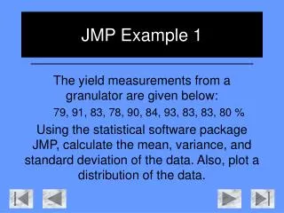
JMP Example 2 Say you take 5 measurements for the yield from a granulator and find the mean measurement. You repeat this process 50 times, to generate a distribution of the data. It can be shown that using 10 or 20 measurements in the first step will give greater accuracy and less variability. Use the data given in MS Excel to make distributions in JMP. Note the change in the shape of the distributions with an increase in the individual sample size, n.
Open JMP, as demonstrated in the last example. Select the “New Data Table”.
Automatically, there is only one column on the Data Table. We need to add 2 more, since we have 3 sets of data. Left click on the right-most red arrow to toggle the column settings.
There are a series of different functions you can carry out on the columns. For this example, we need to add multiple columns.
To add columns to the Data Table, we select the “Add Multiple Columns…” tab.
Here, we may add as many columns as we need. We need three columns in total.
Now we have the three columns; but we need to change their titles. Highlight all of the column title boxes.
This time, we will select the “Column Info…” tab. Note we can change more than just the title here.
The “Column Settings” Window will allow you to change things like the width of the column and the number of rows in the column. Highlight the column name to change it. Repeat for each column.
The “Column Settings” Window will allow you to change things like the width of the column and the number of rows in the column. Highlight the column name to change it. Repeat for each column.
The “Column Settings” Window will allow you to change things like the width of the column and the number of rows in the column. Highlight the column name to change it. Repeat for each column.
The “Column Settings” Window will allow you to change things like the width of the column and the number of rows in the column. Highlight the column name to change it. Repeat for each column. Then press OK.
We also need to add the actual data from MS Excel. To add just one row, double left click on the first box in the left-most Column.
This is the data set with which you are supplied in MS Excel. Highlight the data as shown. Hold the control key “Ctrl” on your keyboard, and press the “C” key on your keyboard. This copies the highlighted data.
When back in JMP, hold down the “Ctrl” key as before, and press “V”. This will paste the data in JMP. Note: Make sure you have all the row highlighted before you do this. Otherwise it will not work.
Similarly to Example 1, we want to use the “Distribution” capability in JMP.
Since we have 3 Columns, we have 3 different data sets upon which we can choose to model the distribution. Select the first one, entitled “Yield (%) with 5 Samples,” and press the “Y, Columns” button.
The distribution of that column will then be drawn. Repeat for all columns required.
The distribution of that column will then be drawn. Repeat for all columns required.
The distribution of that column will then be drawn. Repeat for all columns required.
The distribution of that column will then be drawn. Repeat for all columns required.
The distribution of that column will then be drawn. Repeat for all columns required.
You will then have the three distributions. However, the objective is to compare each distribution. As was shown in the previous example, alter the range and increments of the distributions so that they are all equally weighted on the plots. You may also apply the use of a reference line in the same window. If you need to adjust the graphs further, use the “Grabber” on the toolbar.
Here would be a valid comparison on the three distributions. Note the Box Plot, a common form of distribution summary, over the histograms. The longer the box plot, the larger the variance. You might say the plot of the yield with 20 samples tends more towards a Gaussian (or normal) distribution (a.k.a. the Central Limit Theorem).