Download
1 / 20
210 likes | 318 Views
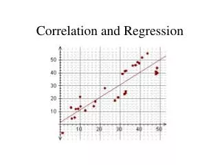
Correlation and Regression. SCATTER DIAGRAM. The simplest method to assess relationship between two quantitative variables is to draw a scatter diagram. From this diagram we notice that as age increases there is a general tendency for the BP to increase. But this does not

E N D
SCATTER DIAGRAM The simplest method to assess relationship between two quantitative variables is to draw a scatter diagram From this diagram we notice that as age increases there is a general tendency for the BP to increase. But this does not give us a quantitative estimate of the degree of the relationship
CORRELATION COEFFICIENT The correlation coefficient is an index of the degree of association between two variables. It can also be used for comparing the degree of association in different groups • For example, we may be interested in knowing whether the degree of association between age and systolic BP is the same (or different) in males and females • The correlation coefficient is denoted by the symbol ‘r’ • ‘r’ ranges from -1 to +1
High values of one variable tend to occur with high values of the other (and low with low) In such situations, we say that there is a positive correlation High values of one variable occur with low values of the other (and vice-versa) we say that there is anegative correlation
A NOTE OF CAUTION Correlation coefficient is purely a measure of degree of association and does not provide any evidence of a cause-effect relationship It is valid only in the range of values studied Extrapolation of the association may not always be valid Eg.: Age & Grip strength
r measures the degree of linear relationship • r = 0 does not necessarily mean that there is no relationship between the two characteristics under study; the relationship could be curvilinear Spurious correlation : The production of steel in UK and population in India over the last 25 years may be highly correlated
r does not give the rate of change in one variable for changes in the other variable Eg: Age & Systolic BP - Males : r = 0.7 Females : r = 0.5 From this one should not conclude that Systolic BP increases at a higher rate among males than females
PROPERTY OF CORRELATION COEFFICIENT Correlation coefficient is unaffected by addition / subtraction of a constant or multiplication / division by a constant to all the values of X and Y Corr. Coeff. between X & Y = 0.7 ,, X+10 & Y-6 = 0.7 ,, 5X & 2Y = 0.7 If the correlation coefficient between height in inches and weight in pounds is say, 0.6, the correlation coefficient between height in cm and weight on kg will also be 0.6
COMPUTATION OF THE CORRELATION COEFFICIENT Sum n = 7 Covariance (XY)
UNIVARIATE REGRESSION Regression :Method of describing the relationship between two variables Use : To predict the value of one variable given the other
SAMPLE DATA SET Patient No. Age (X) Sys BP (Y) 1 45 150 2 48 153 3 46 148 4 45 150 5 46 147 6 48 153 7 46 149 8 55 159 9 51 157 10 56 160 11 53 158 12 60 165 13 53 157 14 54 158 15 49 154 BP = Response (dependent) variable; Age = Predicator (independent) variable
REGRESSION MODEL We can perform a “regression of BP on age”, to derive a straight line that gives an estimated value of BP for any given age. • The general equation of a linear regression line is • Y = a + bX + e • Where, a = Intercept • b = Regression coefficient • e = Statistical error
CALCULATIONS Estimated from the observed values of Age (X) and BP (Y) by least square method b gives the change in Y for a unit change in X a is the value of Y when X = 0, which may not be meaningful always
TEST OF SIGNIFICANCE FOR b Null hypothesis : Test statistic t = Where, The value given under(1) follows a t-distribution with (n-2) df
ASSUMPTIONS 1. The relation between the two variables should be linear 2. The residuals should follow a Normal distribution with zero mean and constant variance
PRECAUTIONS • 1. Adequate sample size should be ensured • Prediction should be made within the range of the • observed values. No extrapolation should be attempted • The equation Y = a + bX should not be used • to predict X for a given Y • 4. Model adequacy should be verified
RESULTS OF REGRESSION ANALYSIS • -------------------------------------------------------------------------------------- • Ind. variable Reg Coeff. SE t P-value • -------------------------------------------------------------------------------------- • Age 1.08 0.08 14.16 < 0.0001 • Constant 100.34 • -------------------------------------------------------------------------------------- • R2 = 93.99% 94% • Systolic BP = 100.34 + 1.08 Age • 95% CI for b = b ± 1.96 SE(b) = 1.08 ± 1.96 x 0.08 • = (0.92, 1.24)
INTERPRETATIONS • 1. Change in age by one year results in a change of • 1.08 mm Hg in Sys. BP • 2. When age = 0, BP = 100.34, which is absurd • BP of a 50 year old individual is • 100.24 + 1.08 x 50 = 154.34 154 mm Hg • 4. 94% of the variation in BP is explained by age alone
MULTIPLE LINEAR REGRESSION The response variable is expressed as a combination of several predictor variables Eg. 0.147 & 1.024 are regression coefficients for ht. and wt. Indicate the increase in for an increase of 1 cm in ht. and 1 kg in wt., respectively
LOGISTIC REGRESSION • Response variable - Presence or absence of some condition • We predict a transformation of the response variable • instead of the actual value of the variable • Data : Hypertension, Smoking (X1) , Obesity(X2) & Snoring (X3) • Which of the factors are predictors of hypertension? • Logit (p) = -2.378 - 0.068 X1 + 0.695 X2 + 0.872 X3 The probability can be estimated for any combination of the three variables Also, we can compare the predicated probability for different groups, e.g., Smokers and Non-smokers