Download
1 / 5
50 likes | 290 Views
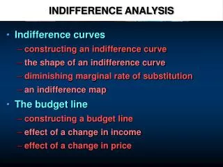
Indifference Curve Analysis of Demand Appendix 3A. U. Consumers attempt to maximize happiness, or utility: U(F, E) over food and entertainment Subject to an income constraint : Y = P F •F + P E •E Graph in 3-dimensions. U o. E. U o. F. U2. U1. F. Uo.

E N D
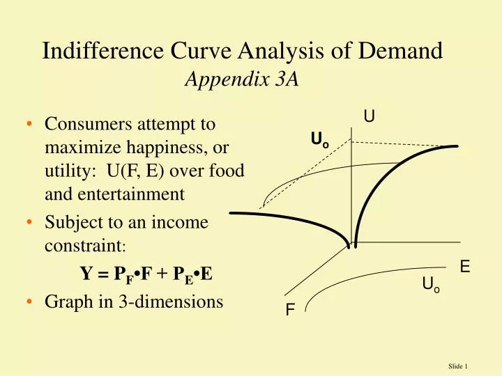
Indifference Curve Analysis of DemandAppendix 3A U • Consumers attempt to maximize happiness, or utility: U(F, E) over food and entertainment • Subject to an income constraint: Y = PF•F + PE•E • Graph in 3-dimensions Uo E Uo F
U2 U1 F Uo Consumer Choice - assume consumers can rank preferences, that more is better than less (nonsatiation), that preferences are transitive, and that individuals have diminishing marginal rates of substitution. Then indifference curves slope down, never intersect, and are convex to the origin. 9 7 6 convex 5 6 7 E give up 2F for one E
Uo U1 F Indifference Curves • We can "derive" a demand curve graphically from maximization of utility subject to a budget constraint. As price falls, we tend to buy more due to (i) theIncome Effect and (ii) the Substitution Effect. c a b E PE demand E
Consumer Choice & Lagrangians • The consumer choice problem can be made into a Lagrangian • Max L = U(F, E) - {PF•F + PE•E - Y } i) L / F = U/F - PF = 0 MUF= PF ii) L / E = U/E-PE = 0 MUE = PE iii) PF•F+ PE•E - Y = 0 • Equations i) and ii) are re-arranged on the right-hand-side after the bracket to show that the ratio of MU’s equals the ratio of prices. This is the optimality condition for optimal consumption }
Optimal Consumption Point • Rearranging we get the Optimality Condition: • MUF / PF = MUE / PE “the marginal utility per dollar in each use is equal” • Lambda is the marginal utility of money SupposeMU1 = 20, and MU2 = 50 and P1 = 5, and P2 = 25 are you maximizing utility?