Download
1 / 83
830 likes | 976 Views
Simulation of initial uncertainties using singular vectors (SVs) and an ensemble of analyses (EDA) (EC/TC/PR/RB-L3). Roberto Buizza European Centre for Medium-Range Weather Forecasts (http://www.ecmwf.int/staff/roberto_buizza/). Outline. The old SV-based ECMWF EPS

E N D
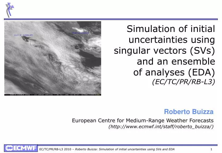
Simulation of initial uncertainties using singular vectors (SVs) and an ensemble of analyses (EDA) (EC/TC/PR/RB-L3) Roberto Buizza European Centre for Medium-Range Weather Forecasts (http://www.ecmwf.int/staff/roberto_buizza/)
Outline • The old SV-based ECMWF EPS • Ensemble Data Assimilation characteristics • The new EDA-SVINI Ensemble Prediction System • EDA-based perturbations and singular vectors
Definition of the perturbed ICs NH SH TR Products 1 2 50 51 ….. 1. The operational ECMWF Ensemble Prediction System • The operational version of the EPS includes 51 forecasts with resolution: • TL639L62 (~32km, 62 levels) from day 0 to 10 • TL319L62 (~64km, 62 levels) from day 10 to 15 (32 at 00UTC on Thursdays). • Initial uncertainties are simulated by adding to the unperturbed analyses a combination of T42L62 singular vectors, computed to optimize total energy growth over a 48h time interval (OTI), and perturbations generated using the new ECMWF Ensembles of Data Assimilation (EDA) system. • Model uncertainties are simulated by adding stochastic perturbations to the tendencies due to parameterized physical processes (SPPT scheme). • The EPS is run twice a day, at 00 and 12 UTC.
1. The old ECMWF Ensemble Prediction System Each ensemble member evolution is given by the time integration of perturbed model equations starting from perturbed initial conditions The model tendency perturbation is defined at each grid point by where rj(Φ,λ) is a random number and μ(p) is a scaling function.
1. The old ECMWF Ensemble Prediction System The EPS initial perturbations do not sample the tropics in an appropriate way, since SVs are computed only for few (up to 6) selected regions and only 10 initial-time SVs are used for each of these regions. The lack of spread in the tropics is evident from a comparison of the ensemble spread and the error of the ensemble-mean. +48h T=0 +120h
1. std/EM of ECMWF 399v255 and 639v319 EPS Over the NH (left), apart for the first 2 days both ensembles have rather good spread-skill relationship, with the new 639v319 showing a better match. Over the Tropics (right), both systems are under-dispersive for the whole forecast range. Can the use of a different set of initial perturbations address this issue? 399v255 (old) 639v319 399v255 (old) 639v319
4. The TIGGE ensembles (updated 12 Apr ‘10) • The 10 TIGGE ensembles use different methodologies to simulate initial-time and model uncertainties. None of them has the right spread for all relevant variables and all forecast steps. The possibility of using a combination of techniques have been explored to improve the ensemble’s reliability. At ECMWF we have been testing the use of Ensemble Data Assimilation perturbations together with SVs.
Outline • The old SV-based ECMWF EPS • Ensemble Data Assimilation characteristics • The new EDA-SVINI Ensemble Prediction System • EDA-based perturbations and singular vectors
2. The ECMWF 4D-Var data-assimilation system The data-assimilation experiments have been run with the following version of the ECMWF data-assimilation/forecasting system: • 12-hour 4-dimentional Variational Data Assimilation System (4D-VAR) • Resolution: • Outer loops at TL511L60 • Inner loops at TL159L60 resolution (50 iter) and TL95L60 (70 iter, reduced phys) • Same set-up as ECMWF early-delivery suite used in operation From each analysis, 10-day TL511L60 forecasts have been run.
2. Ensemble Data Assimilation and Ensemble Prediction • The perturbed analyses are generated by randomly perturbing the observations and the SST, and by running the forecast model with stochastic physics. The random perturbations are defined by sampling a normal distribution with the observation error standard deviation (it is assumed that observations do not have any bias) • Differences between pairs of analyses (and forecast) fields should have the statistical characteristics of analysis (and forecast) error. • Differences between EDA analyses can be used to generate a new set of initial perturbations for the EPS, to further improve the simulation of initial uncertainties. • In data assimilation, the EDA analyses can be used to specify the background errors “of the day”. The ensemble of analyses should indicate where good data should be trusted in the analysis (yellow shading).
2. EDA spread sensitivity to stochastic physics Should the EDA include a model error simulation scheme? The std of EDA generated in 5 configurations: • NOST • BS (back-scatter) • SP1M (rev STPH) • SP1M+BS • Jb (model error from Jb stats) has been compared to the std of a 5-member multi-analysis system.
2. EDA spread sensitivity to stochastic physics This plot shows the std in terms of the kinetic energy at 850 hPa over the Pacific for the 5 EDA configurations: • NOST • BS (back-scatter) • SP1M (rev STPH) • SP1M+BS • Jb (model error from Jb stats) compared to the std of a 5-member multi-analysis system.
2. EDA spread sensitivity to stochastic physics This plot lists the relative difference between the spread (std) of EDA generated in 4 different configurations and of the multi-analysis ensemble with respect to the NOST-EDA for 6 variables over NH.
2. EDA spread sensitivity to stochastic physics This plot lists the relative difference between the spread (std) of EDA generated in 4 different configurations and of the multi-analysis ensemble with respect to the NOST-EDA for 6 variables over the tropics.
2. EDA spread as an indicator of potential analysis error On the 23rd of Dec 2009 a well defined cloud head with a dry slot region ahead of the low centre can be seen in a Meteosat satellite image (left). The area of maximum radial velocity can be seen from the Doppler radar figure from Coruche/Cruz de Leao (east of Lisbon, right). St Cabo Carvoeiro – Min mslp 969 hPa at 0420 UTC – Max wind gust 140 km/h at 0450 UTC Max winds at fixed elevation angle 0.1(quasi-horizontal map) 0400 UTC 0436 UTC 40 – 48 m/s
2. EDA spread as an indicator of potential analysis error The EDA system has been designed to identify areas of potentially large analysis differences. On the 23rd of Dec 2009 a cyclone that developed during the previous 36h in the Atlantic reached Portugal and caused lots of damages. T799 and T1279 analyses showed larger differences in the area of storm development, and forecasts starting from these two analyses differed. Did the EDA identify the Atlantic area where the 799 and the 1279 analyses differ as an area with large spread?
2. EDA spread as an indicator of potential analysis error These plots show the intensity and position error of 639 EPS forecasts started from 799 and 1279 an and valid for 23@00. Results indicate a rather strong sensitivity to the resolution of the unperturbed analysis. How different were the two analyses?
20@00 20@12 2. EDA spread as an indicator of potential analysis error AN_1279 (esuite) AN_799 (ope) diff(1279-799) In the Atlantic region where the small-scale disturbance starts developing, differences between the 1279 (esuite) and the 799 (ope) analyses starts appearing on 20@12.
21@00 21@12 2. EDA spread as an indicator of potential analysis error AN_1279 (esuite) AN_799 (ope) diff(1279-799) The differences between the 1279 (esuite) and the 799 (ope) analyses become larger on 21 Dec.
22@00 22@12 2. EDA spread as an indicator of potential analysis error AN_1279 (esuite) AN_799 (ope) diff(1279-799) After 22@00 the differences between the 1279 (esuite) and the 799 (ope) analyses start decreasing.
2. EDA spread as an indicator of potential analysis error At that time two EPS systems were running (only at 12UTC): • The operational EVO-SVINI 639v319 EPS • The new EDA-SVINI[0.9] 639v319 EPS The comparison of the two systems indicate that overall the EDA-SVINI[0.9] EPS has a larger spread in the area where the 799 and 1279 analyses differ. Differences are particularly larger on 20@12 and 21@12. The following plots compare the MSLP std at initial-time of the EPS forecasts started on 20, 21 and 22 at 12UTC.
2. EDA spread as an indicator of potential analysis error • IC 20@12: • the top row shows the 1279 and the 799 ANs, and their difference. • the bottom row shows the std of the EVO-SVINI and the EDA-SVINI[0.9] EPSs, and their difference.
2. EDA spread as an indicator of potential analysis error • IC 21@12: • the top row shows the 1279 and the 799 ANs, and their difference. • the bottom row shows the std of the EVO-SVINI and the EDA-SVINI[0.9] EPSs, and their difference.
2. EDA spread as an indicator of potential analysis error • IC 22@12: • the top row shows the 1279 and the 799 ANs, and their difference. • the bottom row shows the std of the EVO-SVINI and the EDA-SVINI[0.9] EPSs, and their difference.
2. EDA spread as an indicator of potential analysis error The tropics is the region where the old and the new EPS differ mostly. These figures compare the EVO-SVINI and the EDA-SVINI initial conditions at 12UTC of 20091017 when a tropical depression is present in the analysis at about (130ºE, 15ºN).
Outline • The old SV-based ECMWF EPS • Ensemble Data Assimilation characteristics • The new EDA-SVINI Ensemble Prediction System • EDA-based perturbations and singular vectors
PA_3 PA_1 PA_2 Fig. 1 PA_3 PA_1 PA_2 Fig. 2 3. Ensemble Data Assimilation and Ensemble Prediction • In the past few years, experiments have been performed to test the use of an ensemble of analyses in the EPS in different ways, e.g.: • Using each analysis as a center around which to add SV-based perturbations (fig 1) • Using the ensemble of analyses to generate a set of perturbations to be used in conjunction with SV-based perturbations, starting from either a reference analysis (e.g. the high-resolution unperturbed analysis), or the mean of the ensemble of analyses (fig 2)
3. The EDA- and SV-based ensemble system Each ensemble forecast is given by the time integration of perturbed equations Initial perturbations are defined using perturbed analyses(generated by an ensemble data-assimilation system)and initial SVs with the reference and center analyses defined by
3. The EDA- and SV-based ensemble system Consider e.g. the 00UTC EPS: • In the old EVO-SVINI EPS (top panel), the initial perturbations were generated using a combination of initial-time (blue arrows) and evolved (red arrows) SVs. • In the new EDA-SVINI EPS, the evolved SVs are replaced by EDA-based perturbations are constructed using 6h forecasts of the EDA run for the previous DA cycle (black arrows starting from cyan lines, bottom panel). In both systems, the unperturbed (control) analysis is generated defined by a 6h DA system (green box).
21 00 6 9 12 18 21 00 6 9 3. The EDA- and SV-based ensemble system Note that the EDA-based perturbations are defined by differences between +6h forecasts: This choice is consistent with data-assimilation practice followed when computing Jb statistics. In an operational suite, this allows the EPS to start as soon as the ‘centre’ analysis (e.g. TL1279L91) is available since the day d EDA-based perturbations are generated using +6h forecasts started from the previous EDA cycle.
12 Aj(d-6,+6) 21 00 6 9 3. The EDA-SVINI ensemble systems The choice of using 6h forecasts from the EDA run during the previous DA cycle is also consistent with the fact that the operational 48h-SVs are also computed starting from a 6-hour forecast, i.e. along a t+6h to t+54h trajectory: SVk(d,0) SVk(d,48) 48h-SV traj AT42L62(d-6,6) to (d-6,54) AT42L62(d-6,0) Acenter(d-6,+6) AT42L52(d-6,+54) 21 00 6 9 12 18 Acentre(d,0)=ATL799L91(d,0) EDA cycle Aj(d,0)
3. Ensemble experiments • These results are based on a set of TL399L62 experiments (model cycle 31r2) with the following characteristics: • The EDA analyses have been generated with 12-hour cycling 4D-Var, resolution TL399L91 in the outer-loop, and TL159L91/TL95L91 in the inner loops • The SVs have been computed with a T42L62 resolution, a 48-hour optimisation time interval and a total energy norm (as in the operational system) • The ensemble forecasts have been run up with a TL399L62 resolution, 50 perturbed members, stochastic tendency perturbations and a 10-day forecast length. • The following 4 ensembles configurations are compared: • SVINI: with initial uncertainties defined by initial SVs only • SVEVO-INI: with initial uncertainties defined by evolved and initial SVs • EDA: with initial uncertainties defined by EDA-only initial perturbations • EDA-SVINI: with initial uncertainties defined by EDA- and initial SVs
3. std of EDA, SVINI & EDA-SVINI at t=0 – 22/09/07 EDA SVINI EDA-SVINI EDA-only initial perturbations (left panels) are smaller in amplitudes and in scale than SVINI perturbations (middle panels), but are geographically more global. The right panels show the effect of using both EDA and SVINI perturbations.
3. std of EDA, SVINI & EDA-SVINI at t+12h – 22/09/07 EDA SVINI EDA-SVINI EDA perturbations (left panels) grow less rapidly than SVINI perturbations (middle panels). In the combined EDA-SVINI ensemble, the SVINI component dominates the perturbations’ growth.
3. (MEM5-CON) SVINI EPS - 22/09/2007 t=0 T – (MEM5-CON) U – (MEM5-CON) At t=0, SVINI perturbations (defined by a combination of initial SVs) tend to be localized in space, and to have a larger component in potential than kinetic energy. They also show a westward tilt with high, typical of baroclinically unstable structures. This figure shows two vertical cross sections of the temperature and zonal-wind components of the MEM5 perturbation. 30°N 50°N
3. (MEM5-CON) EDA EPS - 22/09/2007 t=0 T – (MEM5-CON) U – (MEM5-CON) At t=0, EDA perturbations have a smaller scale than the SVINI perturbations, and are less localized in space. They have a similar amplitude in potential and kinetic energy. They tend to have more a barotropic than a baroclinic structure. This figure shows two vertical cross sections of the temperature and zonal-wind components of the MEM5 perturbation. 30°N 50°N
3. Spectra of EDA(3,1,HR) & SVINI EPS – NH t0 The top figure shows the squared amplitude of the SVINI (red) and EDA(3,1,HR) (blue) perturbations in terms of Z500 over NH. The bottom panel shows the same but for T850. Results have been averaged over 13 cases. At initial time, the SVINI perturbations are confined to T42 by construction. The EDA(3,1,HR) perturbations are larger in terms of T850.
3. Spectra of EDA(3,1,HR) & SVINI EPS – NH +12h The top figure shows the squared amplitude of the SVINI (red) and EDA(3,1,HR) (blue) perturbations in terms of Z500 over NH, and of the error of the t+12h control forecast (black). The bottom panel shows the same but for T850. Results have been averaged over 13 cases. At t+12h, the SVINI perturbations have a larger amplitude than the EDA(3,1,HR) perturbations in terms of Z500 (top panel), and a similar amplitude in terms of T850 (bottom panel). Both ensemble spread is smaller than the control error.
3. Spectra of EDA(3,1,HR) & SVINI EPS – NH +24h The top figure shows the squared amplitude of the SVINI (red) and EDA(3,1,HR) (blue) perturbations in terms of Z500 over NH, and of the error of the t+24h control forecast (black). The bottom panel shows the same but for T850. Results have been averaged over 13 cases. At t+24h, the SVINI perturbations have a larger amplitude than the EDA(3,1,HR) perturbations, especially in the wave-numbers where the SVs total energy peaks at optimisation time. On average, the spectra of the SVINI ensemble spread is closer to the spectra of the control error.
3. Spectra of EDA(3,1,HR) & SVINI EPS – NH +120h The top figure shows the squared amplitude of the SVINI (red) and EDA(3,1,HR) (blue) perturbations in terms of Z500 over NH, and of the error of the t+120h control forecast (black). The bottom panel shows the same but for T850. Results have been averaged over 13 cases. At t+120h, the difference in spread between the SVINI and the EDA(3,1,HR) is even more evident. On average, the spectra of the SVINI ensemble spread is very close to the spectra of the control error.
3. Spectra of EDA(3,1,HR) & SVINI EPS – TR 0/12h The top figure shows the squared amplitude of the SVINI (red) and EDA(3,1,HR) (blue) perturbations in terms of T850 over the tropics at initial time. The bottom panel shows the same but for t+12h. Results have been averaged over 13 cases. Results confirm that the SVINI ensemble has too little spread over the tropics.
3. Spectra of EDA(3,1,HR) & SVINI EPS – TR 24/48h The top figure shows the squared amplitude of the SVINI (red) and EDA(3,1,HR) (blue) perturbations in terms of T850 over the tropics at t+24h. The bottom panel shows the same but for t+48h. Results have been averaged over 13 cases. Results confirm that the SVINI ensemble has too little spread over the tropics.
EDA SVINI EDA SVINI 3. std/EM of EDA and SVINI EPS Over the NH (left), the EDA ensemble have smaller spread, and a larger ensemble-mean error from forecast day 3. Over the Tropics (right), the EDA ensemble has larger spread (in terms of T850), and this has a small positive impact on the error of the ensemble-mean, which is slightly smaller between forecast day 2 and 6.
EDA SVINI EDA SVINI 3. RPSS of EDA and SVINI EPS Over the NH (left), the EDA ensemble has a smaller RPSS for T850 probabilistic predictions from forecast day 3, while over the tropics it has a higher RPSS from day 1 (right panel). These results suggest that combining the ensemble of analysis and the initial singular vectors would lead to a better system.
SVEVO-INI EDA-SVINI SVINI EDA SVEVO-INI EDA-SVINI SVINI EDA 3. std/EM of EDA, SVINI, EDA-SVINI & SVEVO-INI EPS The EDA-SVINI ensemble combines the benefits of the EDA and the SV techniques. Over both the NH (left) and the tropics (right), the EDA-SVINI ensemble has a better tuned spread, and the smallest ensemble-mean error (in terms of T850). In the extra-tropics, compared to the SVINI the EDA ensemble severely underestimates the spread, but over the tropics the EDA ensemble has initially a larger spread.
SVEVO-INI EDA-SVINI SVINI EDA SVEVO-INI EDA-SVINI SVINI EDA 3. RPSS of EDA, SVINI, EDA-SVINI & SVEVO-INI EPS The EDA-SVINI ensemble combines the benefits of the EDA and the SV techniques. Over both the NH (left), the EDA-SVINI ensemble is only marginally better than the SVEVO-INI ensemble. But over the tropics (right), the EDA-SVINI ensemble has a higher RPSS. Note that the combination of EDA- and SVINI-based perturbations leads to an ensemble that outperforms one based on EDA-based perturbations only.
Outline • The old SV-based ECMWF EPS • Ensemble Data Assimilation characteristics • The new EDA-SVINI Ensemble Prediction System • EDA-based perturbations and singular vectors
4. EDA-based perturbations and SVs Two conclusions can be drawn from the results shown in the previous section: • Over the extra-tropics, initial perturbations defined using SVs are dominant. EDA-perturbations alone are not sufficient, neither in the short nor in the long forecast range. Without SVs the ensemble is under dispersive. • Over the tropics (30°S-30°N), EDA-based perturbations are dominant. This is not surprising since the current system sub-samples the tropical region: in this region SVs are computed only for few sub-regions. Furthermore only initial-time SVs are used (no evolved SVs). Further evidence of the role of SVs in the extra-tropics comes Observation Simulation Experiments (OSE) that investigated the impact of targeted observations taken in SV-based regions.
Obs IN Obs OUT Sea SV Random t0 →d2 V 4. The impact of targeted data in data-void conditions Consider the following four types of experiments: • SeaIN: control (all obs included) • SeaOUT: no obs in the ocean • SVIN: obs only in SV-target area • RDIN: obs only in random area The comparison of the performance of these experiments can be used to assess the dynamical role of SVs.
RD V SV 4. Ex: ATL and PAC SV-targets for 1/12/03 at 12 UTC Top right: verification region V and area where SVs have maximum final-time total energy. Top left: SV-target (SV) and random (RD) areas defined by 120 grid points (ie the areas where observations were removed in the SVOUT and RDOUT experiments). Bottom: as top but for the Pacific. RD V SV