Download

1 / 27
270 likes | 395 Views
Lecture 8 Software Pipelining. Introduction Problem Formulation Algorithm Reading: Chapter 10.5 – 10.6. I. Example of DoAll Loops. Machine: Per clock: 1 read , 1 write, 1 fully pipelined but 2-cycle ALU with hardware loop op and auto-incrementing addressing mode. Source code:

E N D
Lecture 8Software Pipelining Introduction Problem Formulation Algorithm Reading: Chapter 10.5 – 10.6 CS243: Software Pipelining
I. Example of DoAll Loops CS243: Software Pipelining • Machine: • Per clock: 1 read, 1 write, 1 fully pipelined but 2-cycle ALU with hardware loop op and auto-incrementing addressing mode. • Source code: For i = 1 to n A[i] = B[i]; • Code for one iteration: 1. LD R5,0(R1++) 2. ST 0(R3++),R5 • No parallelism in basic block
Unroll CS243: Software Pipelining 3 1. LD[i] 2. LD[i+1] ST[i] 3. ST[i+1] 2 iterations in 3 cycles 1. LD[i] 2. LD[i+1] ST[i] 3. LD[i+2] ST[i+1] 4. LD[i+3] ST[i+2] 5. ST[i+3] 4 iterations in 5 cycles (harder to unroll by 3) U iterations in 2+U cycles M. Lam
Better Way CS243: Software Pipelining 4 LD[1] loop N-1 times LD[i+1] ST[i] ST[n] • N iterations in 2 + N-1 cycles • Performance of unrolling N times • Code size of unrolling twice M. Lam
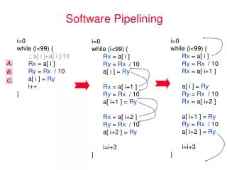
Software Pipelining CS243: Software Pipelining TIME 1. LD0 2. LD1 ST0 3. LD2ST1 4.LD3ST2 Every initiation interval (in this case 1 cycle), Iteration i enters the pipeline (i.e. the first instruction starts) Iteration i-1 (maybe i-x in general) leaves the pipeline (i.e. the last instruction of iteration i-1 finishes)
Unrolling Let’s say you have a VLIW machine with two multiply units for i = 1 to n A[i] = B[i] * C[i];
More Complicated Example Source code: For i = 1 to n D[i] = A[i] * B[i]+ c Code for one iteration: 1. LD R5,0(R1++) 2. LD R6,0(R2++) 3. MUL R7,R5,R6 4. 5. ADD R8,R7,R4 6. 7. ST 0(R3++),R8
Software Pipelined Code CS243: Software Pipelining 1. LD 2. LD 3. MUL LD 4. LD 5. MUL LD 6. ADD LD 7. MUL LD 8. ST ADD LD 9. MUL LD 10. ST ADD LD MUL ST ADD 13. ST ADD 15. 16. ST Unlike unrolling, software pipelining can give optimal result. Locally compacted code may not be globally optimal DOALL: Can fill arbitrarily long pipelines with infinitely many iterations (assuming infinite registers)
Example of DoAcross Loop • LD • MUL • ADD • ST CS243: Software Pipelining Loop: Sum = Sum + A[i]; B[i] = A[i] * c; Software Pipelined Code 1. LD 2. MUL3. ADD LD4. ST MUL 5. ADD 6. ST Doacross loops Recurrences can be parallelized Harder to fully utilize hardware with large degrees of parallelism
II. Problem Formulation S 0 LD 1 MUL2 ADD LD3 ST MUL ADD ST T=2 CS243: Software Pipelining Goals: • maximize throughput • small code size Find: • an identicalrelative schedule S(n) for every iteration • a constantinitiation interval (T) such that • the initiation interval is minimized Complexity: • NP-complete in general
Resources Bound Initiation Interval CS243: Software Pipelining • Example: Resource usage of 1 iteration; Machine can execute 1 LD, 1 ST, 2 ALU per clock LD, LD, MUL, ADD, ST • Lower bound on initiation interval? for all resource i, number of units required by one iteration: ni number of units in system: Ri Lower bound due to resource constraints: maxi ni/Ri
Scheduling Constraints: Resource Iteration 1 LD Alu ST Iteration 2 T=2 LD Alu ST Iteration 3 LD Alu ST Iteration 4 Steady State Time LD Alu ST LD Alu ST T=2 CS243: Software Pipelining RT: resource reservation table for single iteration RTs: modulo resource reservation table RTs[i] = t|(t mod T = i) RT[t]
Scheduling Constraints: Precedence CS243: Software Pipelining for (i = 0; i < n; i++) { *(p++) = *(q++) + c } • Minimum initiation interval? • S(n): Schedule for n with respect to the beginning of the schedule • Label edges with < , d > • = iteration difference, d = delay x T + S(n2) – S(n1) d
Scheduling Constraints: Precedence CS243: Software Pipelining for (i = 2; i < n; i++) { A[i] = A[i-2] + 1; } • Minimum initiation interval? • S(n): Schedule for n with respect to the beginning of the schedule • Label edges with < , d > • = iteration difference, d = delay x T + S(n2) – S(n1) d
Minimum Initiation Interval CS243: Software Pipelining For all cycles c, max c CycleLength(c) / IterationDifference (c)
III. Example: An Acyclic Graph CS243: Software Pipelining
Algorithm for Acyclic Graphs CS243: Software Pipelining Find lower bound of initiation interval: T0 based on resource constraints For T = T0, T0+1, ... until all nodes are scheduled For each node n in topological order s0 = earliest n can be scheduled for each s = s0 , s0 +1, ..., s0 +T-1 if NodeScheduled(n, s) break; if n cannot be scheduled break; NodeScheduled(n, s) • Check resources of n at s in modulo resource reservation table • Can always meet the lower bound if • every operation uses only 1 resource, and • no cyclic dependences in the loop
Cyclic Graphs CS243: Software Pipelining No such thing as “topological order” b c; c b S(c) – S(b) 1 T + S(b) – S(c) 2 Scheduling b constrains c and vice versa S(b) + 1 S(c) S(b) – 2 + T S(c) – T + 2 S(b) S(c) – 1
Strongly Connected Components CS243: Software Pipelining • Astrongly connected component(SCC) • Set of nodes such that every node can reach every other node • Every node constrains all others from above and below • Finds longest paths between every pair of nodes • As each node scheduled, find lower and upper bounds of all other nodes in SCC • SCCs are hard to schedule • Critical cycle: no slack • Backtrack starting with the first node in SCC • increases T, increases slack • Edges between SCCs are acyclic • Acyclic graph: every node is a separate SCC
Algorithm Design CS243: Software Pipelining Find lower bound of initiation interval: T0 based on resource constraints and precedence constraints For T = T0, T0+1, ... , until all nodes are scheduled E*= longest path between each pair For each SCC c in topological order s0 = Earliest c can be scheduled For each s = s0 , s0 +1, ..., s0 +T-1 If SCCScheduled(c, s) break; If c cannot be scheduled return false; Return true;
Scheduling a Strongly Connected Component (SCC) CS243: Software Pipelining SCCScheduled(c, s) Schedule first node at s, return false if fails For each remaining node n in c sl = lower bound on n based on E* su = upper bound on n based on E* For each s = sl , sl +1, min (sl +T-1, su) if NodeScheduled(n, s) break; if n cannot be scheduled return false; Return true;
Anti-dependences on Registers Traditional algorithm ignores them because can post-unroll a1 = ld[i] a2 = a1 + a1; Store[i] = a2; a1 = ld[i+1]; a2 = a1+a1; Store[i+1] = a2;
Anti-dependences on Registers Traditional algorithm ignores them because can post-unroll (or hw support) a1 = ld[i] a2 = a1 + a1; Store[i] = a2; a3 = ld[i+1]; a4 = a3+a3; Store[i+1] = a4; Modulo variable expansion u = maxr (lifetimer /T)
Anti-dependences on Registers The code in every unrolled iteration is identical Not ideal We unroll in two parts of the algorithm Instead, we can run the SWP algorithm for different unrolling factors. For each unroll, we pre-rename the registers but don’t ignore anti-dependences Better potential results But we might not find them
Register Allocation and SWP SWP schedules use lots of registers Different schedules may use different amount of registers Use more back-tracking than described algorithm If allocation fails, try to schedule again using different heuristic Schedule Spills
Conclusions CS243: Software Pipelining • Numerical Code • Software pipelining is useful for machines with a lot of pipelining and numeric code with real instruction level parallelism • Compact code • Limits to parallelism: dependences, critical resource