Download
1 / 45
450 likes | 631 Views
AN INTRODUCTION TO THE OPERATIONAL ANALYSIS OF QUEUING NETWORK MODELS. Peter J. Denning, Jeffrey P. Buzen, The Operational Analysis of Queueing Network Models. ACM Computing Surveys 10(3): 225-261, 1978. Queuing Models. Computer systems contain many queues Ready queue I/O device queues

E N D
AN INTRODUCTION TO THE OPERATIONAL ANALYSISOF QUEUING NETWORK MODELS Peter J. Denning, Jeffrey P. Buzen, The Operational Analysis of Queueing Network Models.ACM Computing Surveys 10(3): 225-261, 1978.
Queuing Models • Computer systems contain many queues • Ready queue • I/O device queues • Message queues • … • Bottlenecks and queuing delays have a major impact on computer system performance • Queuing models capture this impact
Operational Analysis • Operational Analysis • Provides good bounds of performance indices of many computer systems • Only makes verifiable assumptions of behavior of these systems • Is easier to teach and to understand than stochastic analysis
Applications • “Back of the envelope” estimations of system performance • Fast and easy • Validation of results of a simulation study • Checks for reasonableness of results • Communication with non-specialists
Other queuing models • Stochastic models • Also known as Markov models • More powerful • Often make unrealistic assumptions about investigated systems • Disk service times are not exponentially distributed! • Provide surprisingly good estimates of computer system performance
Note • Stochastic models can also be used to estimate • Availability of computer systems:fraction of time system will be operational • Reliability of computer systems:probability that the system will never fail over a time interval of duration t • Essential for real-time systemsand storage systems
Hypothesis testability • All hypotheses made by OA can be tested by • Observing the behavior of actual systems • Over finite time periods
Operational Quantities • Can be • Basic Quantities:Directly measured over a finite observation period • Number of arrivals, … • Derived Quantities:Computed from basic quantities • Server utilization, mean service time, …
A single server • Server has its associated queue • We will treat the server and its queueas a single “black box”
Basic Quantities • T the length of the observation period • A the number of arrivals during the observation period • B the total amount of busy times during the observation period • C the number of completions during the observation period
T A B C
Derived quantities • l = A/T the arrival rate • X = C/T the output rate • U = B/T the utilization • S = B/C the mean service time
Example • Checkout lane: • T = 2 hours • A = 31 customers • B = 108 minutes • C = 30 customers • We have • l = 15.5 customers/hour • …
Utilization law • U = B/T = (C/T )(B/C) = XS • Can compute utilization knowing both • Completion rate • Mean service time When you think about it, it is fairly intuitive
Job flow balance • For most systems, arrivals and completions balance each other over any long observation period • Systems have finite buffers • We will assume that A = C • Can check validity of assumption over any specific observation period • If A = C then U = lS
Steady state • If the system has a steady state, we can define • N = average number of tasks in system • R = average residency of tasks in system • R is also known as the response time
Little’s law • If W is the total time spent by all tasks inside the system over the observation period • Measured in requests × time units • Then • N = W/T • R = W/C • Since W/T = (C/T)(W/C) = XR, N = XR This is an important result
Explanation The green area and the area delimited by thedashed lines have equalsizes Number of tasks in the system N = W/T W Time 0 T
An example • An FBI agent has observed people entering and leaving a secret meeting • Over a period of two hours he has seen 10 people staying an average of 30 minutes each • Having 10 people staying 30 minutes each corresponds to 300 people x minutes • This is the same as having 300/120 = 2.5 people staying over the whole duration of the meeting
Network of servers (I) Open network Arrivals Departures
Network of servers (II) Closed network Arrivals Departures
Operational quantities • Over the observation period, we measure • C = the number of job completions • Ck = the number of tasks completed by device k • We define • X0= C/T = the system throughput • Xk = Ck/T=the output rate at server k • Vk = Ck/C=the visit count at server k
Relations • Ck = VkC • The total number of visits of server k is equal to the number of visits of server k by job completion times the number of job completions • Xk = Vk X0 • The output rate of server k is equal to the number of visits of server k by job completion times the job throughput
Principle of job flow balance • For each device i, the output rate Xiis the same as the total input rates to device i Ai= Ci • True for all observation periods long enough such that |Ai- Ci | << Ci • Output rates Xiare then throughputs
System response time (I) • We define • Nbar = average number of jobs in the system • nbari = average number of jobs at device i • Nbar = Σi nbari
System response time (II) • Applying Little’s law, we have R = Nbar/X0 and nbari = RiXi which we can rewrite nbari = RiViX0 • Hence R = Σi ViRi
Application:Bottleneck analysis • A system has one CPU and one disk drive • It processes transactions such that • VCPU = 12 and SCPU= 5ms • VDisk = 11 and SDISK= 8ms • What is the maximum system throughput?
Bottleneck analysis (cont’d) • Let us compute maximum device throughputs • Maximum XCPU= 1/0.005 = 200 requests/s • Maximum XDisk = 1/0.008 = 125 requests/s • Since Xi = ViX0 • Maximum throughput compatible with CPU workload is 200/12 = 16.7 transactions/s • Maximum throughput compatible with disk workload is 125/11 = 11.4 transactions/s
Bottleneck analysis (cont’d) • The disk is this the bottleneck • It has highest ViSi product • Identifying feature of any bottleneck device • Increasing the system throughput might require • Sharing disk requests with a second disk • Increasing the efficiency of the system I/O buffer Important
Bottleneck analysis (cont’d) • In addition, the maximum throughput of 11.4 transactions/s can only be achieved with a 100% disk utilization • It would result in very large queues at the disk • In practice, we want to limit the disk utilization to 60 to 80%
M Terminals Systems with terminals Whole system
Interactive response time formula • We have • M terminals • Think time Z between the completion of a job and the submission of the next job • Applying Little’s law to the whole system M = (R + Z ) X0 then R = M/X0 – Z Very Important
Problem 1 • A system • Can process up to 5 transactions/s • Has 60 client workstations • Client think time is 5s • Can the system achieve a response time of5 s?
Answer • Applying R = M/X0 – Z, we compute a lower bound for the response time Rmin = M/X0,max – Z = 60/5 – 5 =7 • Our answer is no
Problem 2 • We have • M = 50 terminals • Z = 20 s • R = 4s • What is the system throughput?
Answer • From R = M/X0 – Z, we have X0 = (R + Z)/M Hence X0 = (20 + 4)/50 = 0.48 tasks/s
Problem 3 • Compute the response time of a system knowing the following parameters • M = 25 terminals (users) • Z = 18 s • Vdisk = 20 visits to the single disk per user interaction • Udisk = 0.30 • Sdisk = 25 ms (http://www.owlnet.rice.edu/~elec428/handouts/Op.Analysis.pdf)
Answer • Let us compute first the throughput X0 • Since Xk= Uk/Sk Xdisk= 0.30/0.025 = 12 disk requests/s • Since Xk = Vk X0 , we have X0 = Xk/Vk X0 = 12/20 = 0.6 interactions/s • The response time is then R = M/X0 – Z = 25/0.6 – 18 = 23.7s
Demand • Rather than expressing CPU workloads by the product VCPU SCPU , we can use the total demand of the task DCPU = VCPU SCPU • Since Xk = Uk/Sk and Xk = Vk X0 UCPU /DCPU = XCPU /VCPU= X0
Problem 4 • A computer system has a single disk • It processes tasks with an average CPU demand of 400 ms. • Each task requires 60 disk accesses • Each disk access takes 10 ms • If the CPU utilization is 50%, what are • The system throughput? • The disk utilization?
Answer • X0 = UCPU /DCPU = 0.5/0.4 = 1.25 tasks/s • Since Udisk = Xdisk Sdisk and Xdisk = Vdisk X0 Xdisk= 1.25 x 60 = 75 disk requests/s Udisk= 75 x 0.010 = .75 or 75% (a rather high disk utilization)
Load–dependent behavior • Device service times may depend on number of jobs at device • Disk drives optimize disk accesses • Number of visits to a device may depend on workload • Swap device We did not cover that topic
Resources • http://www.owlnet.rice.edu/~elec428/handouts/Op.Analysis.pdf • Offers a concise summary of the topics that were discussed in class • Peter J. Denning, Jeffrey P. Buzen, The Operational Analysis of Queueing Network Models. ACM Computing Surveys 10(3): 225-261, 1978. • Remains the fundamental text on operational analysis