Download
1 / 33
330 likes | 402 Views
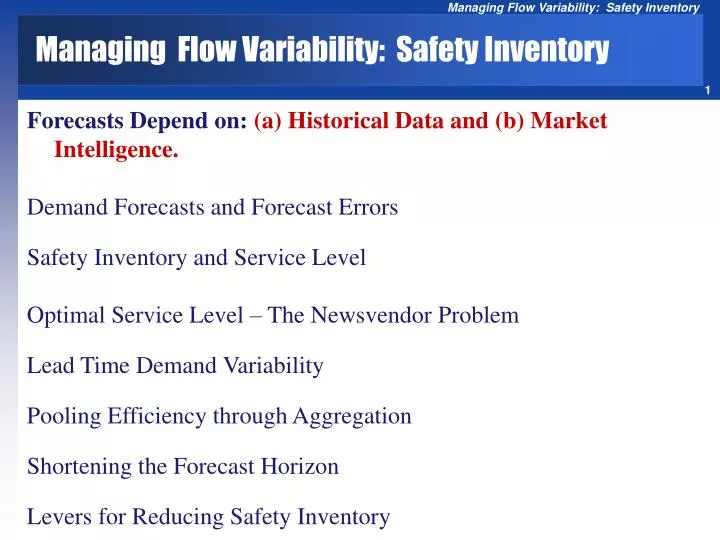
Managing Flow Variability: Safety Inventory. Forecasts Depend on: (a) Historical Data and (b) Market Intelligence. Demand Forecasts and Forecast Errors Safety Inventory and Service Level Optimal Service Level – The Newsvendor Problem Lead Time Demand Variability

E N D
Managing Flow Variability: Safety Inventory Forecasts Depend on: (a) Historical Data and (b) Market Intelligence. Demand Forecasts and Forecast Errors Safety Inventory and Service Level Optimal Service Level – The Newsvendor Problem Lead Time Demand Variability Pooling Efficiency through Aggregation Shortening the Forecast Horizon Levers for Reducing Safety Inventory
Four Characteristics of Forecasts • Forecasts are usually (always) inaccurate (wrong).Because of random noise. • Forecasts should be accompanied by a measure of forecast error.A measure of forecast error (standard deviation) quantifies the manager’s degree of confidence in the forecast. • Aggregate forecasts are more accurate than individual forecasts.Aggregate forecasts reduce the amount of variability – relative to the aggregate mean demand. StdDev of sum of two variables is less than sum of StdDev of the two variables. • Long-range forecasts are less accurate than short-range forecasts.Forecasts further into the future tends to be less accurate than those of more imminent events. As time passes, we get better information, and make better prediction.
Demand During Lead Time is Variable N(μ,σ) Demand of sand during lead time has an average of 50 tons. Standard deviation of demand during lead time is 5 tons Assuming that the management is willing to accept a risk no more that 5%.
Forecasts should be accompanied by a measure of forecast error Forecast and a Measure of Forecast Error
Demand During Lead Time Inventory Demand during LT Time Lead Time
Demand During Lead Time is Variable Inventory Time
Quantity A large demand during lead time Average demand during lead time ROP Safety stock Time LT Safety Stock Safety stock reduces risk of stockout during lead time
Quantity ROP Time LT Safety Stock
Re-Order Point: ROP Demand during lead time has Normal distribution. If we order when the inventory on hand is equal to the average demand during the lead time; then there is 50% chance that the demand during lead time is less than our inventory. However, there is also 50% chance that the demand during lead time is greater than our inventory, and we will be out of stock for a while. We usually do not like 50% probability of stock out We can accept some risk of being out of stock, but we usually like a risk of less than 50%.
Risk of a stockout Average demand Safety stock z-scale Safety Stock and ROP Service level Probability of no stockout ROP Quantity 0 z Each Normal variable x is associated with a standard Normal Variable z x is Normal (Average x , Standard Deviation x) z is Normal (0,1)
Risk of a stockout Average demand Safety stock z Values Service level Probability of no stockout SL z value 0.9 1.28 0.95 1.65 0.99 2.33 ROP Quantity 0 z z-scale • There is a table for z which tells us • Given anyprobability of not exceeding z. What is the value of z • Given anyvalue forz. What is the probability of not exceeding z
μand σ of Demand During Lead Time Demand of sand during lead time has an average of 50 tons. Standard deviation of demand during lead time is 5 tons. Assuming that the management is willing to accept a risk no more that 5%. Find the re-order point. What is the service level. Service level = 1-risk of stockout = 1-0.05 = 0.95 Find the z value such that the probability of a standard normal variable being less than or equal to z is 0.95 Go to normal table, look inside the table. Find a probability close to 0.95. Read its z from the corresponding row and column.
Given a 95% SL 95% Probability The table will give you z Probability z Value using Table Page 319: Normal table 0.05 z Second digit after decimal Z = 1.65 Up to the first digit after decimal 1.6
F(z) z 0 The standard Normal Distribution F(z) F(z) = Prob( N(0,1) <z)
Risk of a stockout Average demand Safety stock Relationship between z and Normal Variable x Service level Probability of no stockout ROP Quantity 0 z z-scale z = (x-Average x)/(Standard Deviation of x) x = Average x +z (Standard Deviation of x) μ = Average x σ = Standard Deviation of x x = μ +z σ
Risk of a stakeout Average demand Safety stock Relationship between z and NormalVariable ROP Service level Probability of no stockout ROP Quantity 0 z z-scale LTD = Lead Time Demand ROP = Average LTD +z (Standard Deviation of LTD) ROP = LTD+zσLTD ROP = LTD + Isafety
Demand During Lead Time is Variable N(μ,σ) Demand of sand during lead time has an average of 50 tons. Standard deviation of demand during lead time is 5 tons Assuming that the management is willing to accept a risk no more that 5%. z = 1.65 Compute safety stock Isafety = zσLTD Isafety = 1.64 (5) = 8.2 ROP = LTD + Isafety ROP = 50 + 1.64(5) = 58.2
Service Level for a given ROP • SL= Prob (LTD ≤ ROP) • LTD is normally distributed LTD = N(LTD, sLTD). • ROP = LTD + zσLTD ROP = LTD + Isafety I safety = z sLTD At GE Lighting’s Paris warehouse, LTD = 20,000, sLTD= 5,000 The warehouse re-orders whenever ROP = 24,000 I safety = ROP – LTD = 24,000 – 20,000 = 4,000 I safety = z sLTD z = I safety / sLTD= 4,000 / 5,000 = 0.8 SL= Prob (Z ≤ 0.8) from Appendix II SL= 0.7881
μ and σ of demand per period and fixed LT Demand of sand has an average of 50 tons per week. Standard deviation of the weekly demand is 3 tons. Lead time is 2 weeks. Assuming that the management is willing to accept a risk no more that 10%. Compute the Reorder Point
μ and σof demand per period and fixed LT R: demand rate perperiod(a random variable) R: Average demand rate perperiod σR:Standard deviation of the demand rate perperiod L: Lead time (a constant number of periods) LTD: demand during the lead time (a random variable) LTD: Average demand during the lead time σLTD:Standard deviation of the demand during lead time
μ and σ ofdemand per period and fixed LT A random variable R:N(R, σR) repeats itself L times during the lead time. The summation of these L random variables R, is a random variable LTD If we have a random variable LTD which is equal to summation of L random variables R LTD = R1+R2+R3+…….+RL Then there is a relationship between mean and standard deviation of the two random variables
μ and σ of demand per period and fixed LT Demand of sand has an average of 50 tons per week. Standard deviation of the weekly demand is 3 tons. Lead time is 2 weeks. Assuming that the management is willing to accept a risk no more that 10%. z = 1.28, R = 50, σR = 3, L = 2 Isafety = zσLTD = 1.28(4.24) = 5.43 ROP= 100 + 5.43
Lead Time Variable, Demand fixed Demand of sand is fixed and is 50 tons per week. The average lead time is 2 weeks. Standard deviation of lead time is 0.5 week. Assuming that the management is willing to accept a risk no more that 10%. Compute ROP and Isafety.
RL R L μ and σ oflead time and fixed Demand per period L: lead time (a random variable) L: Average lead time σL:Standard deviation of the lead time R: Demand per period (a constant value) LTD: demand during the lead time (a random variable) LTD: Average demand during the lead time σLTD:Standard deviation of the demand during lead time
RL R L μ and σ of demand per period and fixed LT A random variable L:N(L, σL) is multipliedby a constant R and generates the random variable LTD. If we have a random variable LTD which is equal to a constant Rtimes a random variables L LTD = RL Then there is a relationship between mean and standard deviation of the two random variables
R + R + R + R + R RL R R R R R R L L Variable R fixed L…………….Variable L fixed R
Lead Time Variable, Demand fixed Demand of sand is fixed and is 50 tons per week. The average lead time is 2 weeks. Standard deviation of lead time is 0.5 week. Assuming that the management is willing to accept a risk no more that 10%. Compute ROP and Isafety. z = 1.28, L = 2 weeks, σL = 0.5 week, R = 50 per week Isafety = zσLTD = 1.28(25) = 32 ROP= 100 + 32
Both Demand and Lead Time are Variable R: demand rate per period R: Average demand rate σR:Standard deviation of demand L: lead time L: Average lead time σL:Standard deviation of the lead time LTD: demand during the lead time (a random variable) LTD: Average demand during the lead time σLTD:Standard deviation of the demand during lead time