Download
1 / 7
70 likes | 203 Views
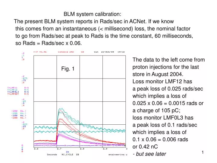
BLM system calibration: The present BLM system reports in Rads/sec in ACNet. If we know this comes from an instantaneous (< millisecond) loss, the nominal factor to go from Rads/sec at peak to Rads is the time constant, 60 milliseconds,

E N D
BLM system calibration: The present BLM system reports in Rads/sec in ACNet. If we know this comes from an instantaneous (< millisecond) loss, the nominal factor to go from Rads/sec at peak to Rads is the time constant, 60 milliseconds, so Rads = Rads/sec x 0.06. The data to the left come from proton injections for the last store in August 2004. Loss monitor LMF12 has a peak loss of 0.025 rads/sec which implies a loss of 0.025 x 0.06 = 0.0015 rads or a charge of 105 pC; loss monitor LMF0L3 has a peak loss of 0.1 rads/sec which implies a loss of 0.1 x 0.06 = 0.006 rads or 0.42 nC - but see later Fig. 1
This shows the same loss monitors LMF0L3 and LMF12 read out by a new digitizer board. The 2nd and 4th trace down are the respective raw data; the 1st and 3rd traces are smoothed over 5 samples. For the new digitizer, 65,536 counts = 10V x 100 pF => 1 count = 0.015 pC LMF12 (2nd trace from bottom) has 300 x 5 = 1500 counts => q total = 22.5 pC (new system) Per R. Shafer, 1 rad = 70 nC, => 0.0015 rads = 105 pC (present system) so I am low by a factor of 5 ??????? Help ! ! ! ! ! ! ! ! Fig. 2 850 peak 0.5 milliseconds/box 1100 peak LMF0L3 300 peak LMF12 400 peak
The conversion used by ACNet to go from volts in the MADC toRads/sec is: Rads/sec = 0.011 x 10 ^ (V/2.39) So a reading of 0.025 Rads/sec => V = 2.39 x log10(0.025/0.011) Volts = 2.39 x 0.36 Volts = 0.86 Volts The plots on the next page show the actual output voltage vs the input current: the offset bias current has a significant effect below 2 Volts - the actual input from the BLM is more like 60 pC.. this helps to reconcile things. As important as this effect, however, is that the losses actually last a long time - and the estimate made by looking at the fast peak is rather misleading. The continuing losses are evident looking at the signal from LMF0L3 as seen in the new system in figure 2. The signal clearly does not return to its baseline after the initial spike. Figure 5 shows the integral of the LMF0L3 signal - a good 2/3 comes after the initial spike.
coulombs Fig. 3 amps Fig. 4 Blue points (and line) are D80 conversion and assume 1 rad/sec = 70 nA 1 r/s 0.1 r/s
Fig. 5 The red is the loss of LMF0L3; the blue is the integral of the LMF0L3 loss (note the factor of 100 in the Scale/ box). The baseline for the integral calculation is estimated using 833(=50 kHz/60) samples from the beginning of the sampling. The loss lasts for 25 milliseconds during which we accumulate (700 - 250) *100 = 45,000 counts, 2/3 of them after the initial spike. 45,000 counts = 0.75 nC 25 milliseconds Integral (multiply scale by 100) peak = 800 Sliding Average of 5 samples
If I look more carefully (ie with present knowledge) at the loss plot of the present BLM, a better estimate of the total loss is the peak x 100 milliseconds. This would imply a total loss of 0.01 Rads or a charge out of the BLM of 0.7 nC to be compared with the 0.75 nC from the new system. The closeness of the two numbers is satisfactory - and I have learnt at least three things. 1) We need to treat low losses reported by the present system a little carefully. 2) It is hard with the present system to distinguish losses that last tens of milliseconds from instantaneous losses - obvious - and these losses show such behavior. 3) The digitizer scale is (at least roughly) correct and we can apply our minds to deciding the proper range. At present the biggest amount of charge we can take in one sample is 1 nC which corresponds to aninstantaneous loss of 0.015 Rads; the largest continuous current we can take is 50 mA which corresponds to a loss of 700 Rads/sec. The latter is much larger than the present system - good; the former is much smaller than the present system - possibly bad. Note that instantaneous in the new system means measured over 20 microseconds; for the present system instantaneous means less than 30 or so milliseconds. The new system as presently arranged can deal with 0.75 Rads in one millisecond. The next page shows the loss rates presently set for aborting in the Tevatron.
Abort limits in the Tevatron are set at ~10 Rads/sec which implies 0.6 rads instantaneous loss. If this loss is actually over one turn, this is 40 times bigger than anything the new system can measure. If it occurs over 1 millisecond or more, the new system can just cope. This has prompted us to consider ways to increase the instantaneous loss capability of the system; see BeamsDoc 1417