Download
1 / 50
560 likes | 890 Views
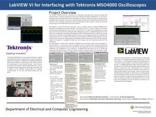
Department of Electrical and Computer Engineering. ECE8231 Digital Signal Processing. Brian M. McCarthy Department of Electrical & Computer Engineering Villanova University. Digital Signal Processing…. Application of DSP - cell phone (2G and after), modem - CD, DVD

E N D
Department of Electrical and Computer Engineering ECE8231 Digital Signal Processing Brian M. McCarthy Department of Electrical & Computer Engineering Villanova University
Digital Signal Processing… Application of DSP - cell phone (2G and after), modem - CD, DVD - computer, simulation… Advantages of using DSP - data compression - undistorted signal transmission - security of data communications - … - representation of signals in discrete-time format - fast & convenient implementation of signal processing systems
Digital Signal Processing … How to use a digital signal to represent an analog signal? How many samples are necessary? What happen if there are no enough samples?
Digital Signal Processing … If the signal is contaminated, how to remove or mitigate the undesired signal component?
Course Arrangement • Text Book: • A. V. Oppenheim, R. W. Schafer, and J. R. Buck, Discrete-Time Signal Processing, 2nd Ed., Prentice Hall, 1999. • Ch. 2 Discrete-Time Signals & Systems • Ch. 3 The z-Transform • Ch. 4 Sampling of Continuous-Time Signals • Ch. 5 Transform Analysis of Linear Time-Invariant • Systems • Ch. 7 Filter Design Techniques • Ch. 8 The Discrete Fourier Transform • Ch. 9 Computation of the Discrete Fourier Transform
Chapter 2 Discrete-Time Signals & Systems
Discrete-Time Signals : Sequences Discrete-time signals are represented mathematically as sequences of numbers. where n is an integer. In practice, such sequences can often arise from periodic sampling of an analog signal. where T is called the sampling period, and fs=1/T is the sampling rate.
Basic Sequences (1) Unit sample sequence (Kronecker Delta function) Unit step sequence Relationships
Basic Sequences (2) Sinusoidal sequence or Complex exponential sequence
Basic Sequences (3) Exponential sequence When a and A are real: A>0, 0<a<1 – decrease with n -1<a<0 – alternative in sign |a|>1 - grows in magnitude
Basic Sequences (4) When a and A are complex: Let A=|A|ejf and a=|a|ejw0, Specifically, when |a|=1, x[n] becomes a complex exponential sequence.
Periodicity of Sinusoidal Sequences and Complex Exponential Sequence A sinusoidal sequence is always periodic (with period 2p) with respect to the frequency. That is, for any integer r, Therefore, we need only consider frequencies in an interval of length 2p, such as –p < w0≤p, or 0 ≤w0 <2p. A periodic sequence is a sequence for which For the underlying sinusoidal sequence, it implies which requires w0N=2pk, for integers N and k. Therefore, the period N is not necessarily equal to 2p /w0. Similar properties hold for complex exponential sequences.
Sinusoidal Sequences with Different Frequencies
Discrete-Time Systems (1) A discrete-time system is defined mathematically as a transformation or operator that maps an input sequence x[n] into a unique output sequence y[n]. T{•}
Discrete-Time Systems (2) The ideal delay system • Memoryless systems A system is referred as memoryless system if the output y[n] at every value of n only depends on the input x[n] at the same value of n. For example,
Discrete-Time Systems (3) • Linear systems The class of linear systems is defined by the principle of superposition. If and a is an arbitrary constant, then the system is linear if and only if (additivity property) (homogeneity or scaling property)
Discrete-Time Systems (4) • Time-invariant systems A time-invariant system is a system for which a time shift or delay of the input sequence causes a corresponding in the output sequence. T{•} T{•}
Discrete-Time Systems (5) • Causality A system is causal if, for every choice of n0, the output sequence value at the index n=n0 depends only on the input sequence value for n≤ n0. Examples: Forward difference system – not causal y[n] = x[n+1] – x[n] Backward difference system - causal y[n] = x[n] – x[n-1]
Discrete-Time Systems (6) • Stability A system is in the bounded input, bounded output (BIBO) sense if and only if every bounded input sequence produces a bounded output sequence. The input x[n] is bounded if there exists a fixed positive finite value Bx such that |x[n]| ≤ Bx <∞ for all n. Stability requires that, for every bounded input, there exists a fixed positive finite value By such that |y[n]| ≤ By <∞ for all n.
Time-invariant T Linear T Linear Time-Invariant Systems A particularly important class of systems consists of those that are linear and time-invariant (LTI). Impulse response If T
Convolution Sum (1) • Convolution Sum Example
Convolution Sum (2) Method 1 For each k for which x[k] has a nonzero value, evaluate x[k] h[n–k] corresponding to the specific x[k]. It equals to the waveform of h[n] multiplied by x[k] and time-shifted by k (shift toward right if k>0, and shift toward left if k<0). 2. Add the resultant sequence values for all k’s to obtain the convolution sum corresponding to the full input sequence x[n].
Convolution Sum (3) • Method 1
Convolution Sum (4) Method 2 For each value n (see *), producing h[n – k]. This is the mirror image of h[k] about the vertical axis shifted by n (shift toward right if n>0, and shift toward left if n<0). Multiply this shifted sequence h[n–k] and the input sequence x[k], and add the resultant sequence values to obtain the value of the convolution at n. Repeat steps 1-2 for different value of n. [* Note the range of n: if x[n] has its nonzero value between x1 and x2, and h[n] has nonzero values between h1 and h2, then x[n]*h[n] has nonzero value between x1+h1 and x2 +h2.]
Convolution Sum (5) • Method 2
Properties of LTI Systems (1) The impulse response is a complete characterization of the properties of a specific LTI system. Convolution operation is commutative x[n]*h[n] = h[n]*x[n] Parallel combination of LTI systems x[n]*(h1[n]+h2[n]) = x[n]*h1[n]+x[n]*h2[n]) h1[n] h1[n]+ h2[n] h2[n]
Properties of LTI Systems (2) Cascade connection of LTI systems h[n]= h1[n]*h2[n] h2[n] h1[n] h1[n] h2[n] h1[n]*h2[n]
Properties of LTI Systems (3) Stability LTI systems are stable if and only if the impulse response is absolutely summable, i.e, if Causality LTI systems are causal if and only if h[n]=0 n<0.
Impulse Responses of Some LTI Systems Ideal delay (stable, causal when nd ≥0) h[n]=d [n – nd] Accumulator (unstable, causal) • Forward difference system (stable, noncausal) h[n] = d [n+1] – d [n] Backward difference system (stable, causal) h[n] = d [n] – d [n –1]
Inverse System If a LTI system has impulse response h[n], then its inverse system, if exists, has impulse response hi[n] defined by the relation h[n]*hi[n] = hi[n]*h[n] =d [n]. Example Accumulator system Backward difference system
Linear Constant-Coefficient Difference Equations (1) An important subclass of LTI systems consists of those systems for which the input x[n] and the output y[n] satisfy an Nth-order linear constant-coefficient difference equation of the form If a0=1, then
Linear Constant-Coefficient Difference Equations (2) • Recursive filter At least one ak≠0 (k = 1, …, N). h[n] has infinite support. Also known as infinite impulse response (IIR) filter. • Non-recursive filter a1, …, aN =0 (no feedback). h[n] has finite support. Also known as finite impulse response (FIR) filter. Example - accumulator One sample delay
Recursive Computation of Difference Equations (1) Consider a system y[n]=ay[n–1]+x[n] with input x[n]=Kd [n] where K is an arbitrary number, and the auxiliary condition y[–1]=c. For n > –1, y[0] = ac + K, y[1] = a2c + aK, … y[n]=an+1c + anK For n < –1 y[–2]=a–1c, y[–3]=a–2c, … y[n]=an+1c In general, y[n]=an+1c+Kanu [n].
Recursive Computation of Difference Equations (2) • In general, it is Noncausal & Nonlinear When K=0, i.e., there is no input, the output y[n] has to be 0 for the system to be causal and linear. However, y[n]=an+1c ≠ 0, unless c=0. • In general, It is not time-invariant When x1[n]=Kd [n–n0], y1[n]=an+1c + anKu[n–n0] ≠ y[n–n0] • When additional initial-rest conditions are satisfied, the system can become LTI and causal. In this example, the initial-rest condition could be c=0.
Recursive Computation of Difference Equations (3) • For a system defined by an Nth-order linear constant-coefficient difference equation, the output for a given input is not uniquely specified. Auxiliary information or conditions are required. • If the auxiliary information is in the form of N sequential values of the output, then the output of the system is uniquely specified. • Linearity, time-invariance, and causality of the system depend on the auxiliary conditions. If an additional condition is that the system is initially at rest, then the system will be LTI and causal.
Summary • Discrete-time signal/system representation • Linear time-invariant (LTI) systems • Impulse response and convolution sum • Stability, causality • Linear constant-coefficient difference equations
Homework Assignments (1) 2.1, 2.4, 2.15, 2.20, 2.22
Analog Signals and Discrete-Time Signals In this example, T=0.025sec, and fs=40Hz.
Discrete-Time Systems (4) • Example of linear systems (accumulator system) • Examples of nonlinear systems
Discrete-Time Systems (6) • Example of time-invariant system - accumulator
Discrete-Time Systems (7) • Example of time-variant system - compressor
Discrete-Time Systems - Examples • Testing for stability or instability y[n]=(x[n])2 is stable because for any |x[n]| ≤ Bx, |y[n]| =|x[n]|2≤ Bx2. So we can choose By = Bx2. • y[n]=log10(|x(n)|) is unstable because when x[n] = 0, y[n]= –∞. • (accumulator) is unstable because when x[n] = u[n], y[n]=(n+1)u[n] which is not bounded.
Summary • Discrete-time signal/system representation • Linear time-invariant (LTI) systems • Impulse response and convolution sum • Stability, causality • Linear constant-coefficient difference equations • Frequency-domain representation of signals/systems
Frequency-Domain Representation of Discrete-Time Signals and Systems (1) • Consider the cases that the input signals are sinusoidal or complex exponential sequences. Complex exponential sequences are eigenfunctions of LTI systems and the response to a sinusoidal input is sinusoidal with the same frequency as the input and with amplitude and phase determined by the system. Let x[n]=e jwnfor –∞ < n < ∞, the corresponding output of an LTI system with impulse response h[n] is
Frequency-Domain Representation of Discrete-Time Signals and Systems (3) • Example – ideal delay y[n] = x (n – nd), h[n] =d (n – nd) If x[n]=e jwn, Alternatively,
Frequency-Domain Representation of Discrete-Time Signals and Systems (2) • The frequency response H(ejw) of discrete-time LTI system is always a periodic function of the frequency variable w with period 2p. • As will be seen later, a broad class of signals can be represented as a linear combination of complex exponentials in the form The corresponding output of a LTI system is