Download
1 / 16
160 likes | 316 Views
Compression. Word document: 1 page is about 2 to 4kB Raster Image of 1 page at 600 dpi is about 35MB Compression Ratio, CR = , where is the number of bits Compression techniques take advantage of: Sparse coverage Repetitive scan lines Large smooth gray areas

E N D
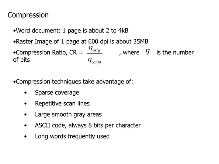
Compression • Word document: 1 page is about 2 to 4kB • Raster Image of 1 page at 600 dpi is about 35MB • Compression Ratio, CR = , where is the number of bits • Compression techniques take advantage of: • Sparse coverage • Repetitive scan lines • Large smooth gray areas • ASCII code, always 8 bits per character • Long words frequently used
Entropy • Entropy is a quantitative term used for amount of information in a string 1.00 0.80 0.60 0.40 0.20 0.00 H(1)+H(0) H(1) H(0) 0.0 0.2 0.4 0.6 0.8 1.0 For N clusters, where li is the length of the ith cluster
Binary Image Compression Techniques • Packing: 8 pixels per byte • Run Length Encoding: Assume 100 dpi, 850 bits per line • encode only the white bits as they are long runs • Top part of a page could be 0(200)111110(3)111110(3) …. • Huffman Coding: use short length codes for frequent messages Encode Decode
0 (2,7) (13,2) 0 (2,7) (13,2) 0 (2,7) (13,2) 0 (2,2) (7,2) (13,2) 0 (2,2) (7,2) (13,2) 0 (2,7) (13,2) 0 (2,2)(7,2)(13,2) 0 (2,2)(7,2)(13,2) 0 0 Bit map: 160 bits 50 numbers in range 0-15 Use 4 bits per number: 200 bits 2 bits per symbol: 100 bits HC: 1.84 x 50 = 92 bits Huffman Encoding
Predictive Coding • Most pixels in adjacent scan lines s1 and s2 are the same • S2’ is the predicted version 2 dimensional prediction • Probabilities gathered from document collections • Tradeoff between context size and table size; Context size of 12 pixels common which uses a 4096 entries table
Group III Fax • White runs and black runs alternate • All lines begin with a white run (possibly length zero) • There are 1728 pixels in a scan line • Makeup codes encode a multiple of 64 bits • Terminating codes encode the remainder (0 to 63) • EOL for each line • CCITT lookup tables • Example, • White run of 500 pixels would be encoded as • 500 = 7x 64 + 52 • Makeup code for 7x 64 is 0110 0100 • Terminating code for 52 is 0101 0101 • Complete code is 0110 0100 0101 0101
Group IV READ b1 b2 Reference Coding a0 a1 a2 • a0 is the reference changing pixel; a1 is the next changing pixel after a0; and a2 is the next changing pixel after a1. • b1 is the first changing pixel on the reference line after a0 and is of opposite color to a0; b2 is the next changing pixel after b1. • To start, a0 is located at an imaginary white pixel point immediately to the left of the coding line. • Follow READ algorithm chart
Group IV READ
Information Retrieval (Typed text documents) • IR goal is to represent a collection of documents were a single document is the smallest unit of information • Typify document content and present information upon request Similarity Measure Requests Documents • OCR translates images of text to computer readable form and IR extracts the text upon request • Inverted Index: Transpose the document-term relationship to a term-document relationship • Remove Stopwords: the, and, to, a, in, that, through, but, etc. • Word Stemming: Remove prefixes and suffixes and normalize
Query 1: recognition or retrievalResponse: 1 2 3 Query 2:sequentially and readableResponse: 3 Query 3:not translateResponse: 2 Query:character and recognition or retrieval
Vector Space Model • Each document is denoted by a vector of concepts (index terms) • If the term is present in the document 1 is placed in the vector • Vector of document 1 from table: (1 1 1 0 1 0 0 1 1 1 1 1 0 0 0 1 1) • Weighting: Favor terms with high frequency in a few documents N = total documents Dfi = no. of docs containing term i Tij = frequency of term i in doc j Document similarity measure between Dj (wi,w2j,…wmj) and Qr (q1r,q2r,..qmr)
Relevance Feedback N = no. of documents in collection R = number of documents relevant to query q N = no. of documents containing t R = no. of relevant documents containing t F =proportion of relevant documents to non-relevant documents in which term occurs F’ = without relevance feedback k = constant, adjusted with collection size c = collection size fi = no. of documents in which term i occurs tij = frequency term i in document j Maxtfj = maximum term frequency in document j
Precision and Recall • Coverage: extent to which system includes relevant documents • Time lag: average time it takes to produce an answer to a search request • Presentation: quality of the output • Effort: energies put forth by user to obtain information sought • Recall: proportion of relevant material received from a query • Precision: proportion of retrieved documents actually relevant Recall= Precision=