Download
1 / 26
260 likes | 412 Views
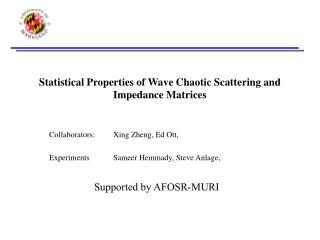
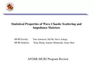
Statistical Properties of Wave Chaotic Scattering and Impedance Matrices. MURI Faculty: Tom Antonsen, Ed Ott, Steve Anlage, MURI Students: Xing Zheng, Sameer Hemmady, James Hart. AFOSR-MURI Program Review. Schematic.

E N D
Statistical Properties of Wave Chaotic Scattering and Impedance Matrices MURI Faculty: Tom Antonsen, Ed Ott, Steve Anlage, MURI Students: Xing Zheng, Sameer Hemmady, James Hart AFOSR-MURI Program Review
Schematic • Coupling of external radiation to computer circuits is a complex processes: apertures resonant cavities transmission lines circuit elements • Intermediate frequency range involves many interacting resonances • System size >> Wavelength • Chaotic Ray Trajectories Integrated circuits cables connectors circuit boards • What can be said about coupling without solving in detail the complicated EM problem ? • Statistical Description ! (Statistical Electromagnetics, Holland and St. John) Electromagnetic Coupling in Computer Circuits
N- Port System N ports • voltages and currents, • incoming and outgoing waves • • • S matrix Z matrix Z(w) , S(w) • Complicated function of frequency • Details depend sensitively on unknown parameters voltage current outgoing incoming Z and S-MatricesWhat is Sij ?
2. Replace exact eigenfunction with superpositions of random plane waves Random amplitude Random direction Random phase 3. Eigenvalues kn2 are distributed according to appropriate statistics: - Eigenvalues of Gaussian Random Matrix Normalized Spacing Random Coupling Model 1. Formally expand fields in modes of closed cavity: eigenvalues kn = wn/c
Port 1 Losses Statistical Model Impedance Other ports RR1(w) Port 2 Radiation Resistance RRi(w) System parameters RR2(w) Dw2n - mean spectral spacing Port 1 Q -quality factor Free-space radiation Resistance RR(w) ZR(w) = RR(w)+jXR (w) wn - random spectrum Statistical parameters win- Gaussian Random variables Statistical Model of Z MatrixFrequency Domain
Model ValidationSummary Single Port Case: Cavity Impedance: Zcav = RR z + jXR Radiation Impedance: ZR = RR + jXR Universal normalized random impedance: z = r + jx Statistics of z depend only on damping parameter: k2/(QDk2) (Q-width/frequency spacing) Validation: HFSS simulations Experiment (Hemmady and Anlage)
Port 1 Losses Zcav = jXR+(r+jx) RR Distribution of reactance fluctuations P(x) Distribution of resistance fluctuations P(r) Dk2 Dk2 Normalized Cavity Impedance with Losses Theory predictions for Pdf’s of z=r+jx
ports h Box with metallic walls Only transverse magnetic (TM) propagate for f < c/2h Ez Hy Hx Voltage on top plate • Anlage Experiments • HFSS Simulations • Power plane of microcircuit Two Dimensional Resonators
Curved walls guarantee all ray trajectories are chaotic Losses on top and bottom plates Moveable conducting disk - .6 cm diameter “Proverbial soda can” HFSS - SolutionsBow-Tie Cavity Cavity impedance calculated for 100 locations of disk 4000 frequencies 6.75 GHz to 8.75 GHz
Theory Theory Comparison of HFSS Results and Modelfor Pdf’s of Normalized Impedance Normalized Reactance Normalized Resistance x r Zcav = jXR+(r+jx) RR
1.05” 1.6” 0. 31” Perturbation Eigen mode Image at 12.57GHz EXPERIMENTAL SETUP Sameer Hemmady, Steve Anlage CSR Circular Arc R=42” Antenna Entry Point 0.310” DEEP 8.5” Circular Arc R=25” SCANNED PERTURBATION 21.4” 17” • 2 Dimensional Quarter Bow Tie Wave Chaotic cavity • Classical ray trajectories are chaotic - short wavelength - Quantum Chaos • 1-port S and Z measurements in the 6 – 12 GHz range. • Ensemble average through 100 locations of the perturbation
Intermediate Loss Low Loss High Loss Theory r x Comparison of Experimental Results and Modelfor Pdf’s of Normalized Impedance
Theory predicts: Uniform distribution in phase Normalized Scattering AmplitudeTheory and HFSS Simulation Actual Cavity Impedance: Zcav = RR z + jXR Normalized impedance : z = r + jx Universal normalized scattering coefficient: s = (z -1)/(z +1) = | s| exp[ if ] Statistics of s depend only on damping parameter: k2/(QDk2)
1 5p/8 3p/8 a) 7p/8 p/8 0 Distribution of Reflection Coefficient ln [P(|s|2)] - p/8 -1 - 3p/8 Theory 1 -1 0 Distribution independent of f |s|2 Experimental Distribution of Normalized Scattering Coefficient s=|s|exp[if]
Zcav = jXR+(r+jx) RR RR = <(r(f1)-1)(r(f2)-1)> XX = <x(f1)x(f2)> RX = <(r(f1)-1 )x(f2)> Frequency Correlations in Normalized ImpedanceTheory and HFSS Simulations (f1-f2)
Eigenvalues of Z matrix q2 Individually x1,2 are Lorenzian distributed Distributions same as In Random Matrix theory q1 Properties of Lossless Two-Port Impedance(Monte Carlo Simulation of Theory Model)
HFSS Solution for Lossless 2-Port Joint Pdf for q1 andq2 Disc q2 Port #1: Port #2: q1
Comparison of Distributed Lossand Lossless Cavity with Ports(Monte Carlo Simulation) Distribution of resistance fluctuations P(r) Distribution of reactance fluctuations P(x) r x Zcav = jXR+(r+jx) RR
Frequency Domain wn- Gaussian Random variables Statistical Parameters wn - random spectrum Time Domain wn- Gaussian Random variables Time Domain Model for Impedance Matrix
Prompt Reflection Delayed Reflection f = 3.6 GHz t = 6 nsec Prompt reflection removed by matching Z0 to ZR Incident and Reflected Pulsesfor One Realization Incident Pulse
Decay of MomentsAveraged Over 1000 Realizations Prompt reflection eliminated Log Scale Linear Scale <V2(t)>1/2 |<V3(t)>|1/3 <V(t)>
t1 = 8.0 10-7 t1 = 5.0 10-7 t1 = 1.0 10-7 Quasi-Stationary Process 2-time Correlation Function (Matches initial pulse shape) Normalized Voltage u(t)=V(t) /<V2(t)>1/2
1000 realizations Incident Pulse Mean = .3163 Histogram of Maximum Voltage |Vinc(t)|max = 1V
Progress • Direct comparison of random coupling model with -random matrix theory P -HFSS solutions P -Experiment P • Exploration of increasing number of coupling ports P • Study losses in HFSS P • Time Domain analysis of Pulsed Signals -Pulse duration -Shape (chirp?) • Generalize to systems consisting of circuits and fields Current Future
Role of Scars? • Eigenfunctions that do not satisfy random plane wave assumption • Scars are not treated by either random matrix or chaotic eigenfunction theory • Semi-classical methods Bow-Tie with diamond scar
Future Directions • Can be addressed -theoretically -numerically -experimentally Features: Ray splitting Losses Additional complications to be added later HFSS simulation courtesy J. Rodgers