Download
1 / 27
270 likes | 385 Views
Variational Principles and Rigidity on Triangulated Surfaces Feng Luo Rutgers University Geometry & Topology Down Under The Hyamfest Melbourne, Australia

E N D
VariationalPrinciplesand Rigidity on Triangulated Surfaces Feng Luo RutgersUniversity Geometry & Topology Down Under The Hyamfest Melbourne, Australia July 17-22, 2011 arXiv:1010.3284
Polyhedral surfaces (S, T, L) Isometric gluing of E2(Euclidean) triangles along edges We also use S2 or H2 triangles.
Eg. Boundary of generic convex polytopes in E3, S3, H3. (S, T) =triangulated surface E ={ all edges in T} V={ all vertices in T} A polyhedral metric Lon (S,T) = edge length function L : E → R s.t., L(ei)+L(ej) > L(ek) In S2 case, we add that the sum of three lengths < 2π.
Curvature Def. The curvature of (S,T, L) isK: V→ R Polyhedral metrics ↔ Riemannian metrics Z ↔ R
Problem: Relationship among metric L, curvature K, topology et al. Eg. 1. Gauss-Bonnet: Eg. 2. Under what condition does K determine the metric L? Eg. 3. Given (S,T), is T a geometric triangulation? i.e., find H2 or E2or S2 metrics on (S, T) with K=0. (discrete uniformization) Eg. 4. What is the meaning of conformality of (S,T,L) and (S, T, L’) ? (discrete Riemann surface) Eg. 5. Given K*:V ->R, find L: E→ R>0 with K* as its curvature. (prescribing curvature problem, shape design in graphics). Eg. 6. What does the Laplace operator tell us about (S,T,L)? (discrete spectral geometry)
Example: Thurston’s circle packing (CP) A(tangential) circle packing (CP) on (S,T) is r: V → R>0. The edge length L: E → R is given by L(uv) = r(u) + r(v)
Thm(Thurston,1978). A E2 or H2CP metric on (S,T) is determined determined up to scaling by its curvature K. Use of CP: calculate Riemann map. Images supplied by D. Gu working with S.T. Yau. Bowers-Stephenson first used CP for brain imaging.
Inversive distance • inversive distance I(C,C’) between circles C, C’ is I(C,C’)=(l2-r2-R2)/(2rR) I(C,C’) is invariant under Mobius transformation. • I(C,C’) in (-1,1) • I(C,C’) =1 • I(C,C’) > 1 Bowers-Stephenson suggested using disjoint circle packing for applications.
Bowers-Stephenson Conjecture (2003) Given (S,T), CP’s on (S,T) with given inversive distance I:E→[1,∞) are determined by their curvature K up to scaling. Thurston, Andreev: CP’s with given inversivedistance I: E →[0,1] are determined by K. Thm 1. Given (S,T) and I: E -> [0, ∞), then CP’s on (S,T) with given inversive distance I are determined by curvature K up to scaling.
Variational Principles (VP) on triangulated spaces Basic example of finite dim VP: F: {n-sided polygons in R2} → R F(P)= area(P) / length2(∂P) maximum of F are the regular n-gons. This is 1.5-dim. We are interested in the 2-dimensional analogy of above.
Variational Principles (VP) on triangulated 3-mfds Schlaefli(1858): for a tetrahedron, w = ∑aidli is closed and S(l) = ∫l w satisfies ∂S/∂li=ai Regge calculus, discrete general relativity (1962) (M3, T) triangulated 3-manifold a polyhedral metric L: E → R>0 Einstein action W(L) = ∑tS(t) - 2π∑e L(e) sum over all tetra t and edges e.
due to Schlafli: ∂S/∂L1=ai W(L) = ∑t S(t) - 2π ∑e L(e) ∂W/∂L1 = a1+a2+…+ak – 2π = -K(e1) a1, a2,…., ak are dihederal angles at e1 K: E → R is the curvature. grad(W) = -K Thm (Regge): Critical points of W(L) are flat metrics.
A 2-D Schlaefli: Colin de Verdiere(1991): w=∑ ai dui is closed, F(u)=∫u w concave in u and ∂F/∂ui=ai ui=ln(ri)
Colin de Verdiere’svariational proof of Thurston’s thm Given (S, T), for u: V → R, define r: V→R by r(v) = eu(v) . W(u) = ∑tF(t, u)-2π∑iui, sum over all triangles t and all ui’s. W: RV → R is concave s.t., ∂W/∂u1=a1+…+ak-2π grad(W) = -K InjectivityLemma If U open convex in Rn, W: U → R is C1 strictly convex, then grad(W): U → Rn is 1-1. W restricted to P={ u | ∑ ui =0} is strictly concave so r to K is 1-1.
Cohen-Kenyon-Propp(2001). For E2 triangles w= ∑ai dui is closed and F(u) = ∫u w is locally convex. the domain of F(u) ={ u | eui+euj>euk} is NOT convex in R3. The injectivity lemma applies locally only.
If the injectivity lemma applies, then Cohne-Kenyon-Propp formula implies: Thm(Rivin) (1994). A E2 polyhedral surface (S,T,L) is determined up to scaling by its φ0 :E →R sending e to a+b. Eg. ai+bi determine tetra φ0 is a new kind of curvature. Curvatures in PL = quantities depending on inner angles.
Q: Can you find all 2D Schlaefli formulas? Thm 2 . For E2 triangles, all 2D schlaefli are (up to scaling) integrations of the closed 1-forms for some λϵ R, • ∫ wλ, wλ = ∑i (∫aisinλ(t) dt/liλ+1) dli (2) ∫ uλ, uλ = ∑i (∫aicotλ(t/2)dt/riλ+1)dri Furthermore, these functions are locally convex/concave. RM. λ=0 corresponds to Colin de Verdiere and Cohne-Kenyon-Propp. RM. There are similar theorems for S2, H2 triangles.
New curvatures Let λ ϵR. For E2, or S2, or H2 polyhedral metric (S, T, L), definediscrete curvatures kλ, ψλ, φλas follows: φλ(e) = ∫aπ/2 sinλ(t) dt + ∫bπ/2 sinλ(t) dt ψλ(e)=∫0(a-x-y)/2cosλ(t) dt + ∫0(b-z-w)/2cosλ(t) dt kλ (v) = (4-m)π/2 -Σa∫aπ/2 tanλ(t/2) dt where a’s are angles at the vertex v of degree m.
Examples kλ(v) = (4-m)π/2 -Σa∫aπ/2 tanλ(t/2) dt • K0= classical K = 2π –angle sum at v φλ(e) = ∫aπ/2 sinλ(t) dt + ∫bπ/2 sinλ(t) dt • φ0 ( e ) = a+b-π : E → R (Rivin) • φ-2(e) = cot(a) + cot(b): E →R discrete cotangent Laplacian operator • φ1 (e) = cos(a) + cos(b), φ-1 (e) = tg(a/2) + tg(b/2) ψ0 –curvature was introduced by G. Leibon 2002
Thm 3. For any λϵR and any (S, T), • a E2 or H2(tangential) CP metric on (S, T) is determined up to scaling by itskλ. (ii) a E2 or S2 polyhedral metric on (S, T) is determined up to scaling by its φλ curvature. • a H2 polyhedral metric on (S, T) is determined by its ψλcurvature. RM 1. (iii) for λ=0 was a theorem of G. Leibon (2002). RM 2. We proved thm 3 (ii) and (iii) in 2007 under some assumptions on λ.
Corollary 4. (a) (Guo-Gu-L-Zeng) Discrete Laplacian determines E2 polyhedral metric (S,T,L) up to scaling. • Discrete Laplacian determines S2 polyhedral metric (S,T,L). RM. We don’t know the answer for H2polyhedral metrics. Eg. A E2 tetrahedron is determined up to scaling by any of the following six tuples: i=1,…,6. (…, ai+bi,.. ) (Rivin) 0 (.., cos(ai)+cos(bi) ,…) 1 (.., tg(ai/2)+tg(bi/2) ,…) -1 (.., cot(ai)+cot(bi) ,..) -2
Proofs of thm 1, 3 use variational principles (VP) Thm 3 uses VP from them 2 Thm 1 uses VP discovered by R. Guo(2009). Guo proved a local rigidity version of thm 1 using his VP. The main problem: domain of the action function is not convex for some λ so the injectivity Lemma does not apply.
Key observation All those locally convex/concave functions in thm 2 and Guo’s action function defined on non-convex open sets can be naturally extended to be convex/concave functions defined in open convex sets. Thus injectivity lemma still applies.
Cohen-Keynon-Propp’s VP and its convex extension w =∑ ai dxi closed w defined on Ω ={ x | } which is not convex in R3 Lemma. ∆3 ={l ϵ R3>0| li+lj >lk} = the space of all E2 triangles. Then a1: ∆3→ R can be extended to a C0-smooth a1*: R3>0 →R s.t., a1 * is constant on each component of R3>0-∆3. Pf.
The extension Extending w from Ω to R3 by w* = ∑ a*i dxi, C0-smooth 1-form w* is closed: ∫ ᵟ w*=0 F*(x) = ∫x w* is well defined. (a) F* is C1 -smooth (b) F* is locally convex on Ω(Cohen-Kenyon-Propp) (c) F* is linear on each component W of R3-Ω since grad(F) on W is a constant by the construction (a)+(b)+(c) imply F* is convex in R3.
Find all non-constant functions W(z1,z2,z3), f(t), g(t) so that for all E2 triangles, We have also proved that Schlaefli in 3D is unique up to scaling in the above sense.