Download
1 / 37
370 likes | 499 Views
Probabilistic tomography. Jeannot Trampert Utrecht University. Is this the only model compatible with the data?. Project some chosen model onto the model null space of the forward operator. Then add to original model. The same data fit is guaranteed!. Deal et al. JGR 1999. True model.

E N D
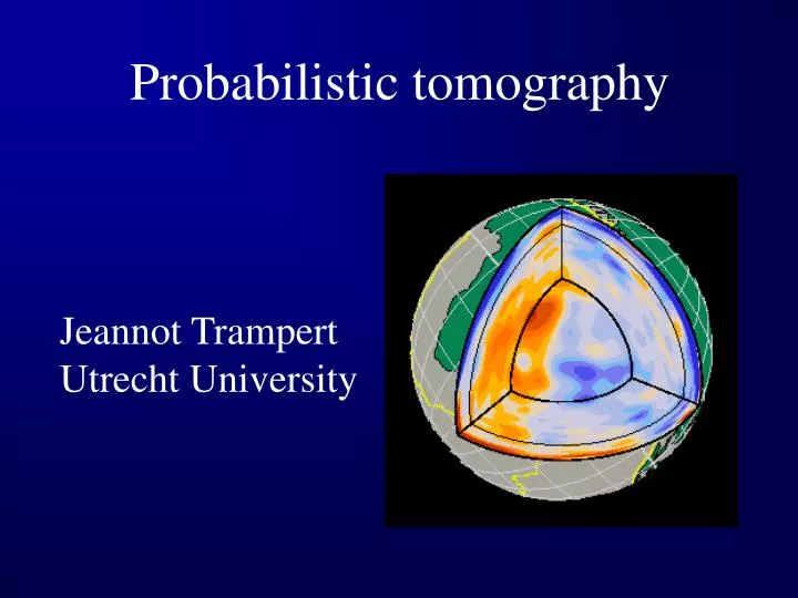
Probabilistic tomography Jeannot Trampert Utrecht University
Is this the only model compatible with the data? Project some chosen model onto the model null space of the forward operator Then add to original model. The same data fit is guaranteed! Deal et al. JGR 1999
True model Forward problem (exact theory) APPRAISAL Model uncertainty Data Estimated model • Inverse problem • (approximate theory, uneven data coverage, data errors) • Ill-posed (null space, continuity) • Ill-conditioned (error propagation)
In the presence of a model null space, the cost function has a flat valley and the standard least-squares analysis underestimates uncertainty. Realistic uncertainty for the given data
Multiple minima are possible if the model does not continuously depend on the data, even for a linear problem. Data Model
Does it matter? Yes! dlnVs dlnVphi dlnrho SPRD6 (Ishii and Tromp, 1999) Input model is density from SPRD6 (Resovsky and Trampert, 2002)
The most general solution of an inverse problem (Bayes, Tarantola)
Only a full model space search can estimate • Exhaustive search • Brute force Monte Carlo (Shapiro and Ritzwoller, 2002) • Simulated Annealing (global optimisation with convergence proof) • Genetic algorithms (global optimisation with no covergence proof) • Sample r(m) and apply Metropolis rule on L(m). This will result in importance sampling of s(m) (Mosegaard and Tarantola, 1995) • Neighbourhood algorithm (Sambridge, 1999) • Neural networks (Meier et al., 2007)
The model space is HUGE! Draw a 1000 models per second where m={0,1} M=30 13 days M=50 35702 years Seismic tomography M = O(1000-100000)
The model space is EMPTY! Tarantola, 2005
The curse of dimensionality small problems M~30 • Exhaustive search, IMPOSSIBLE • Brute force Monte Carlo, DIFFICULT • Simulated Annealing (global optimisation with convergence proof), DIFFICULT • Genetic algorithms (global optimisation with no covergence proof), ??? • Sample r(m) and apply Metropolis rule on L(m). This will result in importance sampling of s(m) (Mosegaard and Tarantola, 1995), BETTER, BUT HOW TO GET A MARGINAL • Neighbourhood algorithm (Sambridge, 1999), THIS WORKS • Neural networks, PROMISING
The neighbourhood algorithm: Sambridge 1999 Stage 1: Guided sampling of the model space. Samples concentrate in areas (neighbourhoods) of better fit.
The neighbourhood algorithm (NA): Stage 2: importance sampling Resampling so that sampling density reflects posterior 2D marginal 1D marginal
Advantages of NA • Interpolation in model space with Voronoi cells • Relative ranking in both stages (less dependent on data uncertainty) • Marginals calculated by Monte Carlo integration convergence check
NA and Least Squares consistency As damping is reduced, LS solution converges towards most likely NA solution. In the presence of a null space, LS solution will diverge, but NA solution remains unaffected.
Finally some tomography! We sampled all models compatible with the data using the Neighbourhood Algorithm(Sambridge, GJI 1999) Data: 649 modes (NM, SW fundamentals and overtones) He and Tromp, Laske and Masters, Masters and Laske, Resovsky and Ritzwoller, Resovsky and Pestena, Trampert and Woodhouse, Tromp and Zanzerkia, Woodhouse and Wong, van Heijst and Woodhouse, Widmer-Schnidrig Parameterization: 5 layers [ 2891-2000 km] [ 2000-1200 km] [1200-660 km] [660-400 km] [400-24 km] Seismic parameters dlnVs, dlnVΦ, dlnρ, relative topography on CMB and 660
Back to density Stage 1 Most likely model SPRD6 Stage 2
Gravity filtered models over 15x15 degree equal area caps • Likelihoods in each cap are nearly Gaussian • Most likely model (above one standard deviation) • Uniform uncertainties • dlnVs=0.12 % • dlnVΦ=0.26 % • dlnρ=0.48 %
Likelihood of correlation between seismic parameters Evidence for chemical heterogeneity Vs-VF Half-height vertical bar corresponds to SPRD6
Likelihood of rms-amplitude of seismic parameters Evidence for chemical heterogeneity RMS density Half-height vertical bar corresponds to SPRD6
The neural network (NN) approach: Bishop 1995, MacKay 2003 • A neural network can be seen as a non-linear filter between some input and output • The NN is an approximation to any function g in the non-linear relation d=g(m) • A training set is used to calculate the coefficients of the NN by non-linear optimisation
The neural network (NN) approach: Trained on forward relation Trained on inverse relation
3) Forward propagating a new datum through the trained network (i.e. solving the inverse problem) dobs 2) Network training: p(m|dobs,w*) 1) Generate a training set: D={dn,mn} Network Input: Observed or synthetic data for training dn Neural Network Network Output: Conditional probability density p(m|dn,w)
Model Parameterization Topography (Sediment) Vs (Vp, r linearly scaled) 3 layers Moho Depth Vpv, Vph, Vsv, Vsh, h 7 layers +- 10 % Prem 220 km Discontinuity Vp, Vs, r 8 layers +- 5 % Prem 400 km Discontinuity
Advantages of NN • The curse of dimensionality is not a problem because NN approximates a function not a data prediction! • Flexible: invert for any combination of parameters • (Single marginal output)
Advantages of NN 4. Information gain Ipost-Iprior allows to see which parameter is resolved Information gain for Moho depth (Meier et al, 2007)
Mean Moho depth [km] Meier et al. 2007 Standard deviation s [km]
Mean Moho depth [km] Meier et al. 2007 CRUST2.0 Moho depth [km]
NA versus NN • NA: joint pdf marginals by integration small problem • NN: 1D marginals only (one network per parameter) large problem
Advantage of having a pdf Quantitative comparison
Mean models of Gaussian pdfs, compatible with observed gravity data, with almost uniform standard deviations:dlnVs=0.12 % dlnVΦ=0.26 % dlnρ=0.48 %
Thermo-chemical • Parameterization: • Temperature • Variation of Pv • Variation of total Fe
Ricard et al. JGR 1993 • Lithgow-Bertelloni and Richards Reviews of Geophys. 1998 • Superplumes