Download

1 / 19
230 likes | 563 Views
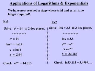
Applications of Logarithms. Lesson 5.8. We will explore applications of the techniques and properties you discovered in the previous lesson.

E N D
Applicationsof Logarithms Lesson 5.8
We will explore applications of the techniques and properties you discovered in the previous lesson. • Logarithms can be used to rewrite and solve problems involving exponential and power functions that relate to the natural world as well as to life decisions. • You will be better able to interpret information about investing money, borrowing money, disposing of nuclear and other toxic waste, interpreting chemical reaction rates, and managing natural resources if you have a good understanding of these functions and problem-solving techniques.
Example A • Recall the pendulum example from Lesson 5.4. The equation y =1.25 + 0.72(0.954)x-10 gave the greatest distance from a motion sensor for each swing of the pendulum based on the number of the swing. • Use this equation to find the swing number when the greatest distance will be closest to 1.47 m. Explain each step.
On the 35th swing, the pendulum will be closest to 1.47 m from the motion sensor.
Example B • Eva convinced the mill workers near her home to treat their wastewater before returning it to the lake. She then began to sample the lake water for toxin levels (measured in parts per million, or ppm) once every five weeks. Here are the data she collected.
Eva hoped that the level would be much closer to zero after this much time. Does she have evidence that the toxin is still getting into the lake? Find an equation that models these data that she can present to the mill to prove her conclusion.
The scatter plot of the data shows exponential decay. So the model she must fit this data to is y = k + abx , where k is the toxin level the lake is dropping toward.If k is 0, then the lake will eventually be clean. If not, some toxins are still being released into the lake. If k is 0, then the general equation becomes y = abx. Take the logarithm of both sides of this equation.
In this equation, c and d are the y-intercept and slope of a line, respectively. So the graph of the logarithm of the toxin level over time should be linear. Let w represent the week and T represent the toxin level.
The graph of (w, log T) shown is not linear. This tells Eva that if the relationship is exponential decay, k is not 0. From the table, it appears that the toxin level may be leveling off at 52 ppm. Subtract 52 from each toxin-level measurement to test again whether (w, log T) will be linear.
The graph of (w, log(T -52)) does appear linear, so Eva can be sure that the relationship is one of exponential decay with a vertical translation of approximately 52. She now knows that the general form of this relationship is y = 52 + abx.
You could now use the same process as in Lesson 5.4 to solve for a and b, but the work you’ve done so far allows you to use an alternate method. Start by finding the median-median line for the linear data (w, log(T 52)).
Cooling • In this investigation you will find a relationship between temperature of a cooling object and time. • Connect a temperature probe to your calculator or a data collector and set it up to collect 18 data points over 180 seconds, or 1 data point every 10 seconds. Heat the end of the probe by placing it in hot water or holding it tightly in the palm of your hand. When it is hot, set the probe on a table so that the tip is not touching anything and begin data collection.
Let t be the time in seconds, and let p be the temperature of the probe. While you are collecting the data, draw a sketch of what you expect the graph of (t, p) data to look like as the temperature probe cools. Label the axes and mark the scale on your graph. Did everyone in your group draw the same graph? Discuss any differences of opinion. • Plot the data in the form (t, p) on an appropriately scaled graph. Your graph should appear to be an exponential function. Study the graph and the data, and guess the temperature limit, L. You could also use a second temperature probe to measure the room temperature, L.
Subtract this limit from your temperatures and find the logarithm of this new list. Plot data in the form (t, log(p L)). If the data are not linear, then try a different limit. • Find the equation that models the data in the previous step, and use this to find an equation that models the (t, p) data in Step 3. Give the real-world meanings of the values in the final equation.
Median-Median Line: y=-0.006949x+0.879754 • Therefore, log(P-22)=-0.0069x+0.8798 • (P-22)=10-0.0069x+0.8798 • P=22+10-0.0069x+0.8798 • P=22+(10-0.0069)x •100.8798 P=22+7.582 (0.98)x The temperature limit is 22°C. The approximate change between the original temperature and the limit is 7.582, and 0.98 is the percentage of this change that occurs each second.