Download
1 / 19
190 likes | 327 Views
Bayesian Methods II: Model Comparison. “Get your facts first, then you can distort them as much as you please”. Mark Twain. Combining Systematic and measurement Errors. Hubble Distance Determination Problem:. H 0 = 70 km/sec/Mpc - Hubble Constant (errors 10 later)

E N D
Bayesian Methods II: Model Comparison “Get your facts first, then you can distort them as much as you please” Mark Twain
Combining Systematic and measurement Errors Hubble Distance Determination Problem: • H0 = 70 km/sec/Mpc - Hubble Constant (errors 10 later) • vm = (100 5) 103 km/sec – recession velocity of galaxy • What is the PDF for the galaxy distance x ? For a Parameter estimation problem: p(x|D,I) p(x| I) p(D|x,I) Assume a uniform prior p(x|I). (Improper prior with infinite range is fine for parameter fitting in this case.) We assume the Likelihood p(D|x,I) is given by a Gaussian PDF representing the error function data-model: (vm-H0x). For simplicity, let us call this error Gaussian Gv(x, H0)distributed about vm with = 5 103.
Combining Systematic and measurement Errors Now we consider 4 separate cases for our prior of H0: CASE1: Assume H0 = 70 km/sec/Mpc (with no error) p(x|D,I) p(x| I) p(D|x,I) = constant Gv(x ,H0) CASE2: Assume H0 = 70 10 km/sec/Mpc with Gaussian prior GH(H0) p(x|D,I) = dH0 p(x, H0 |D,I) p(x| I) dH0 p(H0 | I)p(D|x, H0 I) = p(x| I) dH0GH(H0) Gv(x ,H0)
Hubble Distance PDFs Case 1 Case 2
Combining Systematic and measurement Errors Now we consider 4 separate cases for our prior of H0: CASE3: Assume H0 = 70 20 km/sec/Mpc with uniform prior 90 p(x|D,I) = dH0 p(x, H0 |D,I) 50 90 p(x| I) dH0 p(H0 | I)p(D|x, H0 I) 50 90 p(x| I) dH0 constant Gv(x ,H0) 50 CASE4: Assume H0 = 70 20 km/sec/Mpc with Jeffreys prior 90 p(x|D,I) = dH0 p(x, H0 |D,I) 50 90 p(x| I) dH0 p(H0 | I)p(D|x, H0 I) 50 90 p(x| I) dH0 (1/ H0 ln(90/50)) Gv(x ,H0) 50
Hubble Distance PDFs Case 1 Case 2 Case 3 Case 4
Two basic classes of Inference 1. Model Comparison Which of two or more competing models is the most probable given our present state of knowledge? • Competing models may have free parameters • Models may vary in complexity (some with more free parameters) • Generally, model comparison is not concerned with finding values • Free parameters are usually Marginalized out in the analysis. 2. Parameter Estimation Given a certain model, what is the probability density function for each of its free parameters? • Suppose model M has free parameters f and A • We wish to find p( f | D, M, I) and p( A | D, M, I) • p( f | D, M, I) is known as the Marginal Posterior Distribution for f
Model Comparison: the Odds Ratio I = M1 + M2 + M3 + ... Mn Bayes Theorem: p(Mi | I) p(D|Mi ,I) p(Mi |D, I) = p(D| I) We introduce the Odds Ratio: Oij = p(Mi |D, I) / p(Mj |D, I) p(Mi | I) p(D|Mi I) = p(Mj | I) p(D|Mj I) p(Mi | I) The factor Bij is known as the Bayes Factor. Bij p(Mj | I) Prior Odds Ratio Prior Likelihood
From Odds Ratio to Probabilities If the Odds ratio for model M1is Oi1 , how to get probabilities? Nmod ip(Mi |D, I ) = 1 Divide through by p(M1 |D, I ) & rearrange: Nmod 1 p(Mi |D, I ) Nmod =i = i Oi1 p(M1 |D, I) p(M1|D, I ) Now by definition Oi1 = p(Mi |D, I) / p(M1 ,|D,I) Rearranging: p(Mi |D, I) = Oi1 p(M1 ,|D,I) Oi1 p(Mi |D, I) = j Oj1 O21 1 For only 2 models: p(M2 |D, I) = = 1 + O21 1 + 1/O21
Occam’s Razor Quantified “Entia non sunt multilicanda praeter necessitatem” (entities must not be multiplied beyond necessity) Consider a comparison between two models, M0 and M1: William of Ockham (1285-1349) M1 = f(θ) - one free parameter M0 has fixed θ=θ0- zero free parameters We have no prior reason to prefer either model (Prior odds ratio = 1.0) To compare models we compute the Bayes Factor B10 in favor of M1 over M0 p(D|M1 I) L (M1) B10 = = p(D|M0 I) L (M0)
Occam’s Razor Quantified L(Θ) = p(D|Θ,M1,I) θ = Θ p(θ|M1,I)=1/Δθ- Prior p(D|θ,M1,I)=L (θ) - Likelihood Characteristic Width δθ of the likelihood is defined: δθ dθ p(D|θ, M1 ,I) = p(D|Θ, M1 ,I) δθ Δθ 1/Δθ Then the likelihood for M1 is: L (M1) =p(D|M1,I) Δθ = dθ p(θ|M1 ,I)p(D|θ, M1 ,I) = dθp(D|θ, M1 ,I) 1 Δθ δθ δθ p(D|Θ, M1 ,I) =L (Θ) Δθ Δθ
The Occam Factor The likelihood for the more complicated M1 is: δθ δθ L (M1) =p(D|M1,I) p(D|Θ, M1 ,I) =L (Θ) Δθ Δθ For the simple model M0 there is no integration to marginalize out any parameters, and so: L (M0) =p(D|M0 ,I) = p(D|θ0 ,M1 ,I) = L (θ0) Therefore our Bayes factor in favor of M1 over M0 is: Ωθ L (M1) L (Θ) δθ B10 = Occam Factor for parameter θ L (M0) L (θ0) Δθ Suppose our model M1 has two free parameters θ and φ: L (M1) =p(D|M1,I) Lmax Ωθ Ωφ(Occam factors multiply)
Spectral Line Revisited Hypothesis Space: M1 Gaussian emission line Channel 37 M2 No real signal, only noise. As Before: Noise is Gaussian with n = 1 M1 predicts signal { } -(i - 0)2 Tfi = T exp 2L2 Where: 0 = 37 & L = 2 (channels) Prior estimates of T from 0.1 to 100 M2 predicts signal = 0.0
Spectral Line Model Comparison p(M1 | D, I) p(M1 | I) p(D|M1 I) p(M1 | I) = O12 = B12 p(M2 | I) p(M2 | D, I) p(M2 | I) p(D|M2 I) Set Prior Odds Ratio = 1 (then O12 = B12) For model M1 we need to marginalize over T p(D| M1, I) = dTp(T| M1,I) p(D| T, M1 ,I) Prior Likelihood Prob. Per log interval PDF Jeffreys Calculate odds ratio for both to contrast Jeffreys and Uniform priors. Uniform Jeffreys Uniform
Spectral line model comparison We already calculated the likelihood P(D|T, M1, I) in the previous lecture: di = Tfi + ei i P(D|M1,T,I) = P(E1,E2,E3...En||M1,T,I) = P(Ei||M1,T,I) { } For Gaussian Noise N -(di - Tfi)2 i 1 exp = 2n2 nsqrt(2) { } -i(di - Tfi)2 exp = n-N (2)-N/2 2n2
Spectral line model comparison So for the Uniform Prior case we have: Tmax { } -i(di - Tfi)2 1 P(D|M1,I) = n-N (2)-N/2 dT exp ΔT 2n2 Tmin = 1.131 10-38 Now: p(D|M1,I) Lmax(M1)ΩT and Lmax(M1)= 8.520 10-37 Then we have an Occam factor for the uniform prior ΩT = 0.0133 For the Jeffreys Prior case we have: Tmax { } -i(di - Tfi)2 n-N (2)-N/2 1 P(D|M1,I) = dT exp ln(Tmax /Tmin) T 2n2 Tmin = 1.239 10-37 The Occam factor for the Jeffreys prior ΩT = 0.145
Spectral line model comparison The likelihood for the no-signal M2 model P(D|T, M2 , I) is simply the sum of the Gaussian noise terms. { } -i di 2 exp P(D|M2,T,I) = n-N (2)-N/2 2n2 = 1.133 10-38 M2 has no free parameters, and hence no Occam factor.
Spectral line models: final odds Uniform Prior Odds Ratio : 1.131 10-38 O12 = = 0.9985 1.133 10-38 1 Probability: p(M1 |D, I) = = 0.4996 1 + 1/O12 (odds influenced by low Occam factor ΩT = 0.0133) Although Lmax(M1) /Lmax(M2) 75 Jeffreys Prior Odds Ratio: 1.239 10-37 = 10.94 1.133 10-38 1 Probability: p(M1 |D, I) = = 0.916 1 + 1/O12 p(M2 |D, I) = 0.084
The Laplace Approximation We have an un-normalized pdf P*(x) whose normailzation constant is: Taylor expand the logarithm of P about its peak: where Now we can approximate P*(x) by an unnormalized Gaussian: And we can approximate the normalizing constant Zp by the Gaussian normalization: