Download
1 / 40
400 likes | 599 Views
CSCI-1680 Network Layer: Intra-domain Routing. Rodrigo Fonseca. Based partly on lecture notes by David Mazières , Phil Levis, John Jannotti. Administrivia. Clarification on grading Must pass each of the 3 components assignments, homeworks , exams. Today. Intra-Domain Routing

E N D
CSCI-1680Network Layer:Intra-domain Routing Rodrigo Fonseca Based partly on lecture notes by David Mazières, Phil Levis, John Jannotti
Administrivia • Clarification on grading • Must pass each of the 3 components • assignments, homeworks, exams
Today • Intra-Domain Routing • Next class: Inter-Domain Routing
Routing • Routing is the process of updating forwarding tables • Routers exchange messages about routers or networks they can reach • Goal: find optimal route for every destination • … or maybe a good route, or any route (depending on scale) • Challenges • Dynamic topology • Decentralized • Scale
Scaling Issues • Every router must be able to forward based on any destination IP address • Given address, it needs to know next hop • Naïve: one entry per address • There would be 108 entries! • Solutions • Hierarchy (many examples) • Address aggregation • Address allocation is very important (should mirror topology) • Default routes
IP Connectivity • For each destination address, must either: • Have prefix mapped to next hop in forwarding table • Know “smarter router” – default for unknown prefixes • Route using longest prefix match, default is prefix 0.0.0.0/0 • Core routers know everything – no default • Manage using notion of Autonomous System (AS)
Internet structure, 1990 • Several independent organizations • Hierarchical structure with single backbone
Internet structure, today • Multiple backbones, more arbitrary structure
Autonomous Systems • Correspond to an administrative domain • AS’s reflect organization of the Internet • E.g., Brown, large company, etc. • Identified by a 16-bit number • Goals • AS’s choose their own local routing algorithm • AS’s want to set policies about non-local routing • AS’s need not reveal internal topology of their network
Inter and Intra-domain routing • Routing organized in two levels • Intra-domain routing • Complete knowledge, strive for optimal paths • Scale to ~100 networks • Today • Inter-domain routing • Aggregated knowledge, scale to Internet • Dominated by policy • E.g., route through X, unless X is unavailable, then route through Y. Never route traffic from X to Y. • Policies reflect business agreements, can get complex • Next lecture
Network as a graph • Nodes are routers • Assign cost to each edge • Can be based on latency, b/w, queue length, … • Problem: find lowest-cost path between nodes • Each node individually computes routes
Basic Algorithms • Two classes of intra-domain routing algorithms • Distance Vector • Requires only local state • Harder to debug • Can suffer from loops • Link State • Each node has global view of the network • Simpler to debug • Requires global state
Distance Vector • Local routing algorithm • Each node maintains a set of triples • <Destination, Cost, NextHop> • Exchange updates with neighbors • Periodically (seconds to minutes) • Whenever table changes (triggered update) • Each update is a list of pairs • <Destination, Cost> • Update local table if receive a “better” route • Smaller cost • Refresh existing routes, delete if time out
Calculating the best path • Bellman-Ford equation • Let: • Da(b) denote the current best distance from a to b • c(a,b) denote the cost of a link from a to b • Then Dx(y) = minz(c(x,z) + Dz(y)) • Routing messages contain D • D is any additive metric • e.g, number of hops, queue length, delay • log can convert multiplicative metric into an additive one (e.g., probability of failure)
B’s routing table DV Example
Adapting to Failures G, 3, D • F-G fails • F sets distance to G to infinity, propagates • A sets distance to G to infinity • A receives periodic update from C with 2-hop path to G • A sets distance to G to 3 and propagates • F sets distance to G to 4, through A G, 2, D G, 2, F G, 1, G G, 3, A G, 1, G
Count-to-Infinity • Link from A to E fails • A advertises distance of infinity to E • B and C advertise a distance of 2 to E • B decides it can reach E in 3 hops through C • A decides it can reach E in 4 hops through B • C decides it can reach E in 5 hops through A, … • When does this stop?
Good news travels fast • A decrease in link cost has to be fresh information • Network converges at most in O(diameter) steps B 1 4 1 A C 10
Bad news travels slowly • An increase in cost may cause confusion with old information • May form loops B 12 4 1 A C 10
How to avoid loops • IP TTL field prevents a packet from living forever • Does not repair a loop • Simple approach: consider a small cost n (e.g., 16) to be infinity • After n rounds decide node is unavailable • But rounds can be long, this takes time • Distance vector based only on local information
Better loop avoidance • Split Horizon • When sending updates to node A, don’t include routes you learned from A • Prevents B and C from sending cost 2 to A • Split Horizon with Poison Reverse • Rather than not advertising routes learned from A, explicitly include cost of ∞. • Faster to break out of loops, but increases advertisement sizes
Warning • Split horizon/split horizon with poison reverse only help between two nodes • Can still get loop with three nodes involved • Might need to delay advertising routes after changes, but affects convergence time
Link State Routing • Strategy: • send to all nodes information about directly connected neighbors • Link State Packet (LSP) • ID of the node that created the LSP • Cost of link to each directly connected neighbor • Sequence number (SEQNO) • TTL
Reliable Flooding • Store most recent LSP from each node • Ignore earlier versions of the same LSP • Forward LSP to all nodes but the one that sent it • Generate new LSP periodically • Increment SEQNO • Start at SEQNO=0 when reboot • If you hear your own packet with SEQNO=n, set your next SEQNO to n+1 • Decrement TTL of each stored LSP • Discard when TTL=0
Calculating best path • Djikstra’s single-source shortest path algorithm • Each node computes shortest paths from itself • Let: • N denote set of nodes in the graph • l(i,j) denote the non-negative link between i,j • ∞ if there is no direct link between i and j • C(n) denote the cost of path from s to n • s denotes yourself (node computing paths) • Initialize variables • M = {s} (set of nodes incorporated thus far) • For each n in N-{s}, C(n) = l(s,n) • R(n) = n if l(s,n) < ∞, – otherwise
Djikstra’s Algorithm • While N≠M • Let w ∈(N-M) be the node with lowest C(w) • M = M ∪ {w} • Foreachn ∈ (N-M), if C(w) + l(w,n) < C(n) • then C(n) = C(w) + l(w,n), R(n) = R(w) • Example: D: (D,0,-) (C,2,C) (B,5,C) (A,10,C)
Distance Vector vs. Link State • # of messages (per node) • DV: O(d), where d is degree of node • LS: O(nd) for n nodes in system • Computation • DV: convergence time varies (e.g., count-to-infinity) • LS: O(n2) with O(nd) messages • Robustness: what happens with malfunctioning router? • DV: Nodes can advertise incorrect path cost • DV: Others can use the cost, propagates through network • LS: Nodes can advertise incorrect link cost
Metrics • Original ARPANET metric • measures number of packets enqueued in each link • neither latency nor bandwidth in consideration • New ARPANET metric • Stamp arrival time (AT) and departure time (DT) • When link-level ACK arrives, compute Delay = (DT – AT) + Transmit + Latency • If timeout, reset DT to departure time for retransmission • Link cost = average delay over some time period • Fine Tuning • Compressed dynamic range • Replaced Delay with link utilization • Today: commonly set manually to achieve specific goals
Examples • RIPv2 • Fairly simple implementation of DV • RFC 2453 (38 pages) • OSPF (Open Shortest Path First) • More complex link-state protocol • Adds notion of areas for scalability • RFC 2328 (244 pages)
RIPv2 • Runs on UDP port 520 • Link cost = 1 • Periodic updates every 30s, plus triggered updates • Relies on count-to-infinity to resolve loops • Maximum diameter 15 (∞ = 16) • Supports split horizon, poison reverse
Route Tag field • Allows RIP nodes to distinguish internal and external routes • Must persist across announcements • E.g., encode AS
Next Hop field • Allows one router to advertise routes for multiple routers on the same subnet • Suppose only XR1 talks RIPv2:
OSPFv2 • Link state protocol • Runs directly over IP (protocol 89) • Has to provide its own reliability • All exchanges are authenticated • Adds notion of areas for scalability
OSPF Areas • Area 0 is “backbone” area (includes all boundary routers) • Traffic between two areas must always go through area 0 • Only need to know how to route exactly within area • Otherwise, just route to the appropriate area • Tradeoff: scalability versus optimal routes
Next Class • Inter-domain routing: how scale routing to the entire Internet