Download
1 / 64
650 likes | 746 Views
Use of Regional Models in Impacts Assessments. L. O. Mearns NCAR Colloquium on Climate and Health NCAR, Boulder, CO July 22, 2004.

E N D
Use of Regional Models in Impacts Assessments L. O. Mearns NCAR Colloquium on Climate and Health NCAR, Boulder, CO July 22, 2004
“Most GCMs neither incorporate nor provide information on scales smaller than a few hundred kilometers. The effective size or scale of the ecosystem on which climatic impacts actually occur is usually much smaller than this. We are therefore faced with the problem of estimating climate changes on a local scale from the essentially large-scale results of a GCM.” Gates (1985) “One major problem faced in applying GCM projections to regional impact assessments is the coarse spatial scale of the estimates.” Carter et al. (1994)
But, once we have more regional detail, what difference does it make in any given impacts assessment? What is the added value? Do we have more confidence in the more detailed results?
Elevation (meters) 2500 2250 2000 1750 1500 1250 1000 750 RegCM Topography 0.5 deg. by 0.5 deg. 500 250 0 Elevation (meters) -250 3000 2750 NCAR CSM Topography 2.8 deg. by 2.8 deg. 2500 2250 2000 1750 1500 1250 1000 750 500 250 0
Resolutions Used in Climate Models • High resolution global coupled ocean-atmosphere model simulations are not yet feasible(~ 250 - 300 km) • High resolution global atmospheric model simulations are feasible for time-slice experiments ~ 50-100 km resolution for 10-30 years(~ 100 km) • Regional model simulations at resolution 10-30 km are feasible for simulations 20-50 years(~ 50 km)
Benefits of High Resolution Modeling • Improves weather forecasts (e.g., Kalnay et al. 1998), down to to 10 km and improves seasonal climate forecasts, but more work is needed (Mitchell et al., Leung et al., 2002). • Improves climate simulations of large scale conditions and provides greater regional detail potentially useful for climate change impact assessments • Often improves simulation of extreme events such as precipitation and extreme phenomena (hurricanes).
Regional Climate Modeling • Adapted from mesoscale research or weather forecast models. Boundary conditions are provided by large scale analyses or GCMs. • At higher spatial resolutions, RCMs capture climate features related to regional forcings such as orography, lakes, complex coastlines, and heterogeneous land use. • GCMs at 200 – 250 km resolution provide reasonable large scale conditions for downscaling.
Regional Modeling Strategy Nested regional modeling technique • Global model provides: • initial conditions – soil moisture, sea surface temperatures, sea ice • lateral meteorological conditions (temperature, pressure, humidity) every 6-8 hours. • Large scale response to forcing (100s kms) Regional model provides finer scale response (10s kms)
GLCC Vegetation Reanalysis & GCM Initial and Boundary Conditions Rotated Mercator Projection USGS Topography Regional Climate Model Schematic Hadley & OI Sea Surface Temperatures
Use of Regional Climate Model Results for Impacts Assessments • Agriculture: • Brown et al., 2000 (Great Plains – U.S.) • Guereña et al., 2001 (Spain) • Mearns et al., 1998, 1999, 2000, 2001, 2003, 2004 • (Great Plains, Southeast, and continental US) • Carbone et al., 2003 (Southeast US) • Doherty et al., 2003 (Southeast US) • Tsvetsinskaya et al., 2003 (Southeast U.S.) • Easterling et al., 2001, 2003 (Great Plains, Southeast) • Thomson et al., 2001 (U.S. Pacific Northwest) • Pona et al., (in Mearns, 2001) (Italy)
Use of RCM Results for Impacts Assessments 2 • Water Resources: Leung and Wigmosta, 1999 (US Pacific Northwest) Stone et al., 2001, 2003 (Missouri River Basin) Arnell et al., 2003 (South Africa) Miller et al., 2003 (California) Wood et al., 2004 (Pacific Northwest) • Forest Fires: Wotton et al., 1998 (Canada – Boreal Forest) • Human Health: New York City Health Project (ongoing)
Examples of RCM Use in Climate and Impacts Studies • Precipitation and Hydrology over S. Africa • Water Resources in Pacific Northwest • Agriculture - Southeast US • Human Health – New York • European Prudence Program • New Program – NARCCAP
Regional Climate Modeling and Hydrological Impacts in Southern Africa Arnell et al., 2003, J. Geophys.Research
Observed snow pack , March, 1998 Observed mean annual precipitation Climate Simulations of Western U.S. Strong Effect of TerrainModel ability to resolve terrain features is critical Leung et al., 2004,Climatic Change (Jan.)
Elevation (meters) 2500 2250 2000 1750 1500 1250 1000 750 MM5 Topography 0.5 deg. by 0.5 deg. 500 250 0 Elevation (meters) -250 3000 2750 2500 NCAR/DOE Topography 2.8 deg. by 2.8 deg. 2250 2000 1750 1500 1250 1000 750 500 250 0
Observed and Simulated El Nino Precipitation AnomalyRCM reproduces mesoscale features associated with ENSO events Observation RCM Simulation NCEP Reanalyses
Global and Regional Simulations of SnowpackGCM under-predicted and misplaced snow Regional Simulation Global Simulation
Climate Change Signals Temperature Precipitation PCM RCM
Extreme Precipitation/Snowpack ChangesLead to significant changes in streamflow affecting hydropower production, irrigation, flood control, and fish protection
Special Issue of Climatic Change (60:1-148) Issues in the Impacts of Climatic Variability and Change on Agriculture • Mearns, L. O., Introduction to the Special Issue on the Impacts of Climatic Variability and Change on Agriculture • Mearns, L. O., F. Giorgi, C. Shields, and L. McDaniel, Climate Scenarios for the Southeast US based on GCM and Regional Model Simulations. • Tsvetsinskaya, E., L. O. Mearns, T. Mavromatis, W. Gao, L. McDaniel, and M. Downton,The Effect of Spatial Scale of Climate Change Scenarios on Simulated Maize, Wheat, and Rice Production in the Southeastern United States. • Carbone, G., W. Kiechle, C. Locke, L. O. Mearns, and L. McDaniel, Response of Soybeans and Sorghum to Varying Spatial Scales of Climate Change Scenarios in the Southeastern United States. • Doherty, R. M., L. O. Mearns, R. J. Reddy, M. Downton, and L. McDaniel, A Sensitivity Study of the Impacts of Climate Change at Differing Spatial Scales on Cotton Production in the SE USA. • Adams, R. M., B. A. McCarl, and L. O. Mearns, The Economic Effects of Spatial Scale of Climate Scenarios: An Example From U. S. Agriculture.
Models Employed • Commonwealth Scientific and Industrial Research Organization (CSIRO) GCM – Mark 2 version • Spectral general circulation model • Rhomboidal 21 truncation (3.2 x 5.6); 9 vertical levels • Coupled to mixed layer ocean (50 m) • 30 years control and doubled CO runs • NCAR RegCM2 • 50 km grid point spacing, 14 vertical levels • Domain covering southeastern U.S. • 5 year control run • 5 year doubled CO runs
Domain of RegCM denotes study area + denotes RegCM Grid Point (~ 0.5o) X denotes CSIRO Grid Point (3.2 o lat. 5.6 o long)
RegCM Topography (meters) Contour from 100 to 4000 by 100 (x1)
Climate Change - Δ Temperature (oC) CSIRO RegCM CSIRO RegCM Summer Fall Minimum Temperature Maximum Temperature 7.00 to 10.00 6.00 to 7.00 5.00 to 6.00 4.00 to 5.00 3.00 to 4.00 2.00 to 3.00 1.00 to 2.00 0.00 to 1.00 -1.00 to 0.00
Conclusions Regionalization of the climate change scenarios matters in terms of the economic indicators of the ASM • Shows up in aggregate economic welfare (different orders of magnitude); • Regional patterns of agricultural production are altered; • more spatial variability with RegCM; • Southern states are more negatively affected by RegCM.
Conclusions (Con’t.) • The contrast in economic net welfare based on spatial scale of climate scenarios is similar in magnitude to the economic contrast resulting from use of two very different AOGCM simulations in the US National Assessment.
Modeling the Impact of Global Climate and Regional Land Use Change on Regional Climate and Air Quality over the Northeastern United States C. Hogrefe, J.-Y. Ku, K. Civerolo, J. Biswas, B. Lynn, D. Werth, R. Avissar, C. Rosenzweig, R. Goldberg, C. Small, W.D. Solecki, S. Gaffin, T. Holloway, J. Rosenthal, K. Knowlton, and P.L. Kinney This project is supported by the U.S. Environmental Projection Agency under STAR grant R-82873301
NY Climate & Health Project:Project Components • Model Global Climate • Model and Evaluate Land Use • Model Regional Climate • Model Regional Air Pollution (ozone, PM2.5) • Evaluate Health Impacts (heat, air pollution) • For 2020s, 2050s, and 2080s
Model Setup • GISS coupled global ocean/atmosphere model driven by IPCC greenhouse gas scenarios (“A2” high CO2 scenario presented here) • MM5 regional climate model takes initial and boundary conditions from GISS GCM • MM5 is run on 2 nested domains of 108km and 36km over the U.S. • CMAQ is run at 36km to simulate ozone • 1996 U.S. Emissions processed by SMOKE and – for some simulations - scaled by IPCC scenarios • Simulations periods : June – August 1993-1997 June – August 2053-2057
A Model Look Into the 2050’s • How will modeled temperature and ozone in the northeastern U.S. change under the “A2” (high CO2 growth) scenario (assume constant VOC and NOx emissions)? • How will CMAQ ozone predictions change when IPCC “A2” projected changes in ozone precursor emissions (VOC+8%, NOx+29.5%) are included in the simulation?
Research questions • Health Risk Assessment: • Deaths due to short-term heat exposures • Hospital admissions due to short-term ozone exposures • Development of model linkages • Scale Intercomparison: as we go from 108 -> 36 -> 4km scale, what difference do we see in impact estimates? How do model results compare at different scales for NY metro region.
Global Climate Model NASA-GISS IPCC A2, B2 Scenarios meteorological variables Regional Climate ClimRAMS MM5 reflectance; stomatal resistance; surface roughness heat Public Health Risk Assessment meteorological variables: temp., humidity, etc. Land Use / Land Cover SLEUTH, Remote Sensing Ozone PM2.5 Air Quality MODELS-3 IPCC A2, B2 Scenarios
GCM and RCM Projections
RCMs and Simulation of Extremes Do they do better?
1993 Midwest Summer Flood • Record high rainfall (>200 year event) • Thousands homeless • 48 deaths • $15-20 billion in Damage USHCN Observations J. Pal RegCM
RegCM 1988 Great North American Drought CRU Observations • Driest/warmest since 1936 • $30 billion in Agricultural Damage
Putting spatial resolution in the context of other uncertainties • Must consider the other major uncertainties regarding future climate in addition to the issue of spatial scale – what is the relative importance of uncertainty due to spatial scale? • These include: • Specifying alternative future emissions of ghgs and aerosols • Modeling the global climate response to the forcings (i.e., differences among GCMs)
PRUDENCE Project Multiple AOGCMs and RCMs over Europe: Simulations of Future Climate
Summary of RegCM3Results for A2 and B2 scenariosNested in HADAM3 time-slice • RegCM3 – 50 km • HadAM3 time slice – 100 km • Years – 1961-1990 vs. 2070 –2099 • Control run results • Changes in Climate Giorgi et al., 2004
Emissions Scenarios CO2 Emissions (Gt C) CO2 Concentrations (ppm) A2 A2 B2 B2