Download
1 / 52
520 likes | 647 Views
Lecture 10 Land-Atmosphere Feedback: Observational Studies. …which affects the overlying atmosphere (the boundary layer structure, humidity, etc.). …causing soil moisture to increase. Precipitation wets the surface. …which causes evaporation to increase during subsequent days

E N D
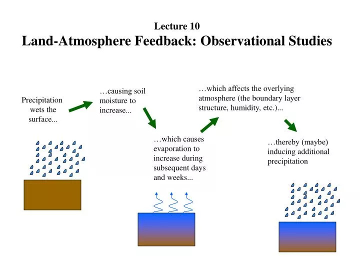
Lecture 10 Land-Atmosphere Feedback: Observational Studies …which affects the overlying atmosphere (the boundary layer structure, humidity, etc.)... …causing soil moisture to increase... Precipitation wets the surface... …which causes evaporation to increase during subsequent days and weeks... …thereby (maybe) inducing additional precipitation
First, some slides from last week… How about AGCM studies that only initialize the soil moisture? (I.e., studies that don’t prescribe soil moisture throughout the simulation period?) Beljaars et al., Mon. Weather Rev., 124, 362-383…. Such studies include Oglesby and Erickson, J. Climate, 2, 1362-1380, 1989. Also: Wet initial- ization Rind, Mon. Weather Rev., 110, 1487-1494. June 1 initialized dry Dry initial- ization Differ- ences
Impact of Soil Moisture Predictability on Temperature Prediction (darker shades of green denote higher soil-moisture impact) …and a study by Schlosser and Milly (J. Hydromet., 3, 483-501, 2002), in which the divergence of states in a series of parallel simulations was studied in detail: Predictability Timescale Estimate (via memory) for soil moisture Actual Predictability Timescale (diagnostics of precipitation show a much weaker soil-moisture impact) Some recent studies have examined the impact of soil moisture initialization on forecast skill (relative to real observations). These will be discussed in the next lecture.
LAND-ATMOSPHERE INTERACTION: IS THERE ANY OBSERVATIONAL EVIDENCE? Findell and Eltahir (1997) provide evidence that soil moisture variations in Illinois affect precipitation, though the evidence is disputed by Salvucci et al. (2002). Evidence that the nature of the boundary layer over land is influenced by variations in soil moisture include the analysis of Betts and Ball (1995): dry soil wet wet soil dry dry dry wet wet
Precipitation 1 6 10 16 21 26 July Impacts on precipitation are much more difficult to identify. Problem: The search for evidence of feedback in nature is limited by scant soil moisture and evaporation data – we have no observational evidence of feedback on precipitation at the large scale. Calculate: Lag-2 autocorrelationbetween precipitation pentads Question: Can we uncover evidence of feedback at the large scale in the observational precipitation record?
Observational data set: “Unified Precipitation Database”, put together by Higgins et al. Daily, ¼ o over the U.S. for 1948-1997 Based on 12000 stations/day (on average) Assembled from: NCD Coop.; RFC daily; NCDC hourly, accumulated to daily Aggregation: Data aggregated to pentads (5 day totals) at 2o x 2.5o. AGCM strategy for interpreting the observations: 1. Identify a feature of interest in the autocorrelation field (or other field). 2. See if the AGCM reproduces this behavior. 3. If so, determine what causes the behavior in the AGCM. 4. Infer that the same mechanisms apply in nature. something of a leap of faith…
July Rainfall: Variance (normalized) Correlations (pentads, twice removed) July Rainfall: Mean July Rainfall: Variance [mm/day] [mm2/day2] [dimensionless] [dimensionless] AGCM AGCM, no feedback Obser- vations 0. 0.12 0.16 0.24 0.50 0.08 -0.24 -0.50 -0.16 -0.12 -0.08 0. 0.5 0.8 1.3 2.0 3.2 5.0 8.0 0.13 0.20 0.32
The observations show a pattern of autocorrelation that is similar in location and timing, though not in magnitude, to that produced by the GCM. Possible reasons: 1. Statistical fluke 2. The pattern is a reflection of something unrelated to land-atmosphere feedback, such as monsoon dynamics, long-term precipitation trends, or SST variability. 3. The pattern does reflect land-atmosphere feedback. Note: if #3 is correct, then an analysis of what controls feedback in the GCM could shed further light on the observations. What might be going on? In the west:high evaporation sensitivity yields low soil moisture memory, and low evaporation yields low impact on rainfall. In the east: consider the evaporation-versus-soil moisture curve: E Where things are wet, evaporation is not sensitive to soil moisture. W
Can we explainwhat controls ac(P) in the GCM? GCM obs correlates with Pn Pn+2 means that Pn Pn+2 Breaks down in western US correlates with correlates with En+2 correlates with wn wn+2 Breaks down in eastern US correlates with Breaks down in western US
Another study: Evidence of Feedback in Observational PDFs Dataset: GPCP monthly precipitation, 1979-2000. Approach: Rank precipitation for a given month into pentiles; determine conditional PDFs of rainfall in the following month for each pentile. Standardize and assume ergodicity to generate the PDFs. Does July rainfall for these years tend to be higher than normal? years with highest June rainfall June rainfall: 4th level June rainfall: 3rd level June rainfall: 2nd level Does July rainfall for these years tend to be lower than normal? years with lowest June rainfall
…but only when land-atmophere feedback in the model is enabled:
Note that the broadness of the PDFs implies that while feedback exists, the prediction skill associated with the feedback may be quite limited.
More Evidence: Historical Temperature Distributions 1. What lies behind the distribution of soil moisture variance? Low rain case: lower limit, soil wants to stay really dry low variance. Intermediate case: no limits, no “absorbing state” high variance. High rain case: upper limit, soil wants to stay really wet low variance 1 0 mean soil moisture (degree of saturation) Soil moisture variance versus mean soil moisture, as simulated by a GCM 1 0 mean soil moisture (degree of saturation)
Evaporation as a function of soil moisture: simplified picture In this regime, evaporation is no longer sensitive to soil moisture variations In this regime, evaporation increases with soil moisture. E/Rnet 0 1 mean soil moisture (degree of saturation)
In this regime, soil moisture variance is translated to a zero evaporation variance In this regime, soil moisture variance is translated to a nonzero evaporation variance E/Rnet 0 1 mean soil moisture (degree of saturation) Evaporation as a function of soil moisture: simplified picture Impact on Evaporation Variance
Variance as a function of mean soil moisture: midlatitude land (AGCM results) s2: W In this regime, soil moisture variance is translated to a zero evaporation variance Soil Moisture In this regime, soil moisture variance is translated to a nonzero evaporation variance E/Rnet s2: E Evaporation 0 1 mean soil moisture (degree of saturation) Mean soil moisture
Variance as a function of mean soil moisture: midlatitude land (AGCM results) s2: W Soil Moisture s2: E Evaporation The surface temperature distribution is strongly correlated with the evaporation distribution. Why? Because more evaporation means more latent cooling of the land surface. s2: T Temperature Mean soil moisture
2. What lies behind the distribution of soil moisture skew? Low rain case: lower limit, positive skew. Intermediate case: no limits, zero skew. High rain case: upper limit, negative skew 1 0 mean soil moisture (degree of saturation) Positive skews are emphasized because precipitation itself is positively skewed. Soil moisture skew versus mean soil moisture, as simulated by a GCM 1 0 mean soil moisture (degree of saturation)
Evaporation as a function of soil moisture: simplified picture Impact on Evaporation Skew Negative Eskew promoted Zero Eskew promoted E/Rnet 0 1 mean soil moisture (degree of saturation)
Skew as a function of mean soil moisture: midlatitude land (AGCM results) Impact on Evaporation Skew Skew: W Soil Moisture Negative Eskew promoted Zero Eskew promoted Skew: E E/Rnet Evaporation 0 1 Mean soil moisture mean soil moisture (degree of saturation)
Skew as a function of mean soil moisture: midlatitude land (AGCM results) Skew: W Soil Moisture Skew: E Evaporation Again, the surface temperature distribution follows the evaporation distribution. (A strong negative correlation.) Negative of Skew: T Temperature Mean soil moisture
Idealized schematic of soil moisture/evaporation impacts on temperature moments maximum of soil moisture variance maximum of temperature variance negative temperature skew positive temperature skew dryer wetter large continental region This behavior is seen clearly in the AGCM. Is it seen in the observations?
maximum of soil moisture variance maximum of temperature variance negative temperature skew positive temperature skew dryer wetter large continental region The U.S. is one such place to look for these features: 1) Relatively clean west-to-east moisture gradient 2) GHCN temperature data spanning close to a century 3) Soil moisture proxies: derived from GSWP2 modeling study, but based on observed precipitation, radiation, etc. soil moisture distribution (degree of saturation)
Temperature Variance (GHCN observations) Dots: estimated high soil moisture variance, from independent GSWP2 analysis
Idealized schematic of soil moisture/evaporation impacts on temperature moments maximum of soil moisture variance maximum of temperature variance negative temperature skew positive temperature skew dryer wetter large continental region
Temperature Skew (observations) dots: high temperature variance (observations)
Binned Results MODEL RESULTS OBSERVATIONS Mean soil moisture Mean soil moisture
maximum of soil moisture variance maximum of temperature variance negative temperature skew positive temperature skew dryer wetter large continental region Summary of Temperature Analysis Soil moisture boundaries and the shape of the evaporation function have a first-order effect on the distributions of the second and third moments of evaporation – and thus temperature – in the AGCM. In the AGCM, these effects place the maximum of temperature variance on the dry side of the maximum of soil moisture variance. They place the maximum of the temperature skew on the wet side of this variance maximum, and they place negative temperature skew on the dry side of this variance maximum. Analysis of observational temperature fields (spanning 100 years, from GHCN) show strong hints of these same features. The geographical distribution of temperature moments in nature appear to be hydrologically controlled at seasonal timescales. Either that, or the agreement with the model results is pure coincidence.
More studies... Some AGCM studies examine the impact of “perfectly forecasted” soil moisture on the simulation of observed extreme events. Examples: Hong and Kalnay (Nature, 408, 842-844, 2000) studied the impact of dry soil moisture conditions on the maintenance of the 1998 Oklahoma-Texas drought. Schubert et al. (see fig. 1 of Entekhabi et al., BAMS, 80, 2043-2058, 1999) demonstrated that their AGCM could only capture the 1988 Midwest drought and the 1993 Midwest flood if soil moistures were maintained dry and wet, respectively.
Key test: Impact of land initialization on forecast skill Other studies have examined the impact of “realistic” soil moisture initial conditions on the evolution of subsequent model precipitation. Studies include: Viterbo and Betts, JGR, 104, 19361-19366, 1999. Also: Douville and Chauvin, Clim. Dyn., 16, 719-736, 2000. Fennessy and Shukla, J. Climate, 12, 3167-3180, 1999.
ATMOSPHERIC CALCULATIONS Time step n+1 ATMOSPHERIC CALCULATIONS Time step n E,H E,H Precip. Precip. Rad. Rad. T,q,… T,q,… Observed Precip. Observed Precip. LAND CALCULATIONS Time step n LAND CALCULATIONS Time step n+1 Detailed description of another recent study of this type (Koster and Suarez, J. Hydromet., 2003) POOR MAN’S LDAS: A study of the impacts of soil moisture initialization on seasonal forecasts At every time step in a GCM simulation, the land surface model is forced with observed precipitation rather than GCM-generated precipitation. The observed global daily precipitation data comes from GPCP and covers the period 1997-2001 at a resolution of 1o X 1o (George Huffman, pers. Comm.) The daily precipitation is applied evenly over the day.
Note: for the “soil moisture initialization” runs, some scaling is required to ensure an initial condition consistent with the AGCM: Essentially, a dry condition for the GPCP forcing run… …is converted to an equivalently dry condition for the AGCM forecast simulation.
Key finding from this study: soil moisture initialization has an impact on forecasted precipitation only when three conditions are satisfied: 1. Strong year-to-year variability in initial soil moisture. 2. Strong sensitivity of evaporation to soil moisture (slope of evaporative-fraction-versus-soil-moisture relationship). 3. Strong sensitivity of precipitation to evaporation (convective fraction).
On average, there is a hint of improvement associated with land moisture initialization
Illustration of point 6: The ensemble mean is off, but some of the ensemble members do give a reasonable forecast
A more “statistically complete” experiment was tried next.... Approach: GLDAS project (NASA/GSFC) using Berg et al. (2003) data Wind speed, humidity, air temperature, etc. from reanalysis Observed precipitation Observed radiation Initial conditions for subseasonal forecasts Mosaic LSM The resulting initial conditions: (1) Reflect observed antecedent atmospheric forcing, and (2) Are consistent with the land surface model used in the AGCM.
1-Month Forecasts Performed Atmosphere not “initialized”. Land initializatized on: May 1 June 1 July 1 Aug. 1 Sept. 1 1979 1980 1981 1992 1993 75 separate 1-month forecasts, each of which can be evaluated against observations. (Note: each forecast is an average over 9 ensemble members.)
We compare all results to a parallel set of forecasts that do not utilize land initialization: the “AMIP” forecasts. The AMIP forecasts do not rely on atmospheric initialization, either. In essence, the AMIP forecasts derive skill only from the specification of SST. Before we evaluate the forecasts, we ask a critical question: what is the maximum predictability possible in this forecasting system? To answer this, we perform an idealized analysis: STEP 1: For each of the 75 forecasted months, assume that the first ensemble member represents “nature”. STEP 2: For each of these months, assume that the remaining 8 ensemble members represent the forecast. STEP 3: Determine the degree to which the “forecast” agrees with the assumed “nature”. STEP 4: Repeat 8 times, each ensemble member in turn taken as “nature”. Average the resulting skill diagnostics.
Regress “forecast” against “observations” to retrieve r2, our measure of forecast skill.
The idealized analysis effectively determines the degree to which atmospheric chaos foils the forecast, under the assumptions of “perfect” initialization, “perfect” validation data, and “perfect” model physics. In other words, it provides an estimate of “maximum possible predictability”.
Where we look for skill is also limited by quality of observations
Areas with adequate idealized predictability and adequate rain gauge density Precipitation Forecast Areas Breadth of areas that can be tested will increase with future improvements in data collection and analysis. Temperature Forecast Areas
FORECAST EVALUATION: PRECIPITATION Without initialization With initialization Differences Idealized differences
FORECAST EVALUATION: TEMPERATURE Without initialization With initialization Differences Idealized differences
What happens when the atmosphere is initialized (via reanalysis) in addition to the land variables? Supplemental 9-member ensemble forecasts, for June only (1979-1993): 1. Initialize atmosphere and land 2. Initialize atmosphere only Warning: Statistics are based on only 15 data pairs! June r2 values, averaged over area of focus AMIP runs: SSTs only SSTs + land initialization + atmosphere initialization SSTs + atmosphere initialization GLDAS runs: SSTs + land initialization