Download
1 / 85
850 likes | 1.02k Views
Overview: A Sampling of Some Recent Computational Modeling Efforts. MA354 – Computational Math Modeling. Cellular Automata Models. Properties, Definition of Cellular Automata. Discretized Space A regular lattice of “nodes”, “sites”, or “cells” Discretized Time

E N D
Overview: A Sampling of Some Recent Computational Modeling Efforts MA354 – Computational Math Modeling
Properties, Definition of Cellular Automata • Discretized Space • A regular lattice of “nodes”, “sites”, or “cells” • Discretized Time • The lattice is a dynamical system updated with “time-steps”. • Discretized States For Each Node • E.g.; binary states
Properties, Definition of Cellular Automata • Universal Rule for Updating Node States • Applied to every node identically • States at time t+1 are based on states at time t • Neighborhood (local) Rule for Updating Node States • New node states are determined by nearby states within the “interaction neighborhood” • Rules may be deterministic or stochastic
Versatility of CA in Biology 1980-1995 • Occular dominance in the visual cortex Swindale 1980 • Tumor Growth Duchting & Vogelssaenger, 1983; Chodhury et al, 1991;Pjesevic & Jiang 2002 • Microtubule Arrays Smith et al, 1984; Hammeroff et al, 1986 • Animal Coat Markings Young 1984, Cocho et al, 1987 • Cell sorting Bodenstein, 1986; Goel & Thompson 1988, Glazier & Graner 1993 • Neural Networks Hoffman 1987 • Nerve and muscle, cardiac function Kaplan et al 1988 • Cell dispersion Othmer, Dunbar, Alt 1988 • Predator Prey Models Dewdney 1988 • Immunology Dayan et al, 1988; Sieburgh et al, 1990; DeBoer et al, 1991 • Angiogenesis Stokes, 1989; Peirce & Skalak 2003 • Cell Differentiation and Mitosis Nijhout et al 1986; Dawkins 1989 • Plant Ecology Moloney et al 1991 • Honey Bee Combs Camazine 1991 • G-protein Activation Mahama et al 1994 • Bacteria Growth Ben-Jacob et al 1994
Versatility of CA in Biology 1995-2005 • Population dynamics Janecky & Lawniczak 1995 • Reaction diffusion Chen, Dawson, Doolen 1995 • Actin Filaments Besseau & Geraud-Guille 1995 • Animal Herds Mogilner & Edelstein-Keshet 1996 • Shell pigmentation Kusch & Markus 1996 • Alignment Cook, Deutsch, Mogilner 1997 • Fruiting Body Formation of Dicty Maree & Hogeweg 2000 • Convergent Extension Zebrafish Zajac, Jones, Glazier 2002 • Fruiting Body Formation Myxobacteria Alber, Jiang, Kiskowski, 2004 • Limb Chondrogenesis Kiskowski et al, 2004; Chaturvedi et al, 2004 • T-cell Synapse Formation Casal, Sumen, Reddy, Alber, Lee, 2005 Cellular Automata Approches to Biological Modeling Ermentrout and Edelstein-Keshet, J. theor. Biol, 1993
Application: Modeling FRAP “Fluorescent Recovery After Photobleaching” Modeling the diffusion of fluorescent molecules and “photobleaching” a region of the lattice to look at fluorescence recovery. 1. Fluorescent molecules diffuse on the lattice. 2. All molecules in Region A are “photobleached” (state changes from ‘1’ to ‘0’). 3. Recovery: remaining flourescent molecules diffuse into Region A randomly.
Application: Modeling FRAP Modeling the diffusion of fluorescent molecules and “photobleaching” a region of the lattice to look at fluorescence recovery.
Limb Development • Cellular Potts Model for cell-cell interactions (cell sorting into clusters that will become bones) • Coupled with a reaction diffusion equation that instructs what shapes the clusters should be
1. Model For Limb Chondrogenesis Reaction Diffusion Developmental Model Based On Reaction Diffusion and Cell-matrix Adhesion. Computational Model and Results “Interaction between reaction-diffusion and cell-matrix adhesion in a CA model for chondrogenic patterning: a prototype study for developmental modeling” Kiskowski, Alber, Thomas, Glazier, Bronstein and Newman, Dev. Biol., to appear.
Reaction-Diffusion Systems Chemical peaks occur in a system with an autocatalytic component (an activator) and a faster-diffusing inhibiting component (an inhibitor). Result: periodic peaks in stripes or spots described by complex Bessel equations. [Meinhardt, 1995]
Limb Formation in vivo • Bone formation is mediated by fibronectin, which links cells together. • As the limb grows, the number of precartilage condensations increases. • Bone formation occurs from the proximal to distal region. http://zygote.swarthmore.edu/limb4.html
Computational Model • Cells on a 2D circular spot on a square lattice • -Simulation of simplified, in vitro model • -quasi-3D • Reaction-Diffusion • Cell-Fibronectin Adhesion
Reaction (Occurs At Each Node Independently) Activation: CA=Activator concentration CB=Inhibitor concentration nc = cell concentration Up-regulation of Inhibitor: Inhibition: InhibitorDecay:
Diffusion • Model Particles: • Cells, Activator, Inhibitor, and Fibronectin • At each time-step, cells, activator molecules and inhibitor molecules diffuse by either: • resting at their current node with probability ps (or ) • moving right, up, left or down with probability (1-ps)/4. As the probability of restingps increases, the diffusion rate of the particle decreases.
Cell-Matrix Adhesion • Cells produce fibronectin at threshold levels of activator. • Fibronectin does not diffuse. • Cells stick to fibronectin with probability pf and un-stick with probability 1-pf. • Once stuck, cells do not diffuse during that time-step. Fibronectin With Stuck Cells Fibronectin
Preliminary Results Reaction diffusion establishes pattern of activator peaks. Activator Peaks Inhibitor Peaks Fibronectin produced at activator peaks slows cell diffusion and cells cluster. Final Cell Distribution Final Fibronectin Distribution
Hybrid Models • a hybrid model contains both discrete (for example, individual cells defined on a lattice) and continuous elements. • These elements must be ‘coupled’ in some way so the model elements interact and exchange information
Phototaxis during the Slug Stage of Dictyostelium discoideum: a Model StudyMarée, Panfilov and Hogeweg Proceedings of the Royal Society of London. Series B. Biological sciences266 (1999) 1351-1360
Example: A Tumor Model Based on Diffusion and Growth with 2 Continuous Fields Model of Dormann & Deutsch, 2002 • Model components similar to that of Düchting and Vogelsaenger, 1983: • Cell divisions based on cell cycle • Added stochastic transitions • Added cell density and nutrient dependence • Two cell types: normal and fast growth • Cell death (necrosis) based on cell cycle • Two continuous fields: • Diffusing chemotactic field secreted by necrotic cells attracts cancer cells • Diffusing nutrient field • 200x200 2D lattice • Results in layered tumor structure.
(a) The tumor is cut in half and recovers. (b) Cell adhesion is lowered and tumor expands. (c) Necrosis rate is increased by 1000%, tumor survives.
Paracrine Signaling Occurs when a cell or tissue produces a factor which acts upon an adjacent tissue.
Mathematical modeling of epithelial-stromal interactions • Modeling Goal • How can we define epithelial and stromal cell rules that • (1) are biologically motivated, • (2) model correct proliferative behavior, • (3) model correct invasive behavior? • Method: Hypothesize a set of simplified biologically motivated rules and use computer simulations to check if they are sufficient to yield expected cell behaviors. • Warning: If successful, we identify rules that are sufficient to explain experimental observations. Discourse between model predictions and further experiments are needed to further validate/refine the model.
Altered Stroma HGF 1 Proliferative Epithelium Invasive Epithelium Normal Epithelium
Altered Stroma Normal Stroma 50% Altered Stroma Invasive Epithelium HGF SDF 1 2 Proliferative Epithelium Invasive Epithelium Normal Epithelium
Hybrid Model • Discrete, Cell-based Component • Cells are modeled as discrete, individual entities in 2D space. • Stromal and epithelial cells: 5 cell types. • Stromal cells are ‘normal’ or ‘altered’. • Epithelial cells are ‘normal’, ‘proliferative’ or ‘invasive’. • Different stromal types secrete different morphogens. • Epithelial cells progress sequentially from normal to proliferative to invasive if there are threshold levels of the required morphogen.
Hybrid Model • Continuous, PDE Component • Morphogen production, diffusion and decay is modeled with the heat equation. • Production rates k1, k2 (s-1) • Diffusion rates D1, D2 • Decay rates kd1, kd2
Simulation Results PIN Invasion
Phase Diagram: Transitions Depend Weakly on Production Levels
The Prisoner’s Dilemma Applied to the Interaction of Black Flies and Their Residents Maria Byrne – Math & Stats John McCreadie – Biology University of South Alabama MAA Local Meeting University of West Florida Friday, November 18th
Prisoner’s Dilemma (Melvin Dresher and Merrill Flood, 1950) • Game Theory: Analysis of decisions made by rational agents in a hypothetical situation with fixed rules (game) where each agent has options that affect themselves and the group (different payoffs). When will cooperative or altruistic behavior be the winning strategy? (Verses uncooperative or ‘cheating’ behavior.)
Prisoner’s Dilemma (Axelrod, 1984) Prisoner’s Dilemma (Melvin Dresher and Merrill Flood, 1950) • Prisoner’s Dilemma • Two Prisoners • Police do not have enough evidence for a conviction. • Prisoner Options (Silence, Defection) • The prisoners can stay silent, in which case they will be sentenced for 1 month on a minor charge. • A prisoner can inform on the other prisoner (defect) in which case that prisoner goes free and the other serves a year in jail. • If both prisoners defect, they both serve 3 months in jail.
Prisoner’s Dilemma (Melvin Dresher and Merrill Flood, 1950) • Payoff Matrix Prisoner A Prisoner B
Prisoner’s Dilemma (Melvin Dresher and Merrill Flood, 1950) • Payoff Matrix – From a Global Perspective Prisoner A Prisoner B
Prisoner’s Dilemma (Melvin Dresher and Merrill Flood, 1950) • Payoff Matrix – From a Global Perspective Prisoner A Prisoner B
Prisoner’s Dilemma (Melvin Dresher and Merrill Flood, 1950) • Payoff Matrix – From a Global Perspective Prisoner A Prisoner B
Prisoner’s Dilemma (Melvin Dresher and Merrill Flood, 1950) • Payoff Matrix – From a Global Perspective Prisoner A Prisoner B
Prisoner’s Dilemma (Melvin Dresher and Merrill Flood, 1950) • Payoff Matrix – From a Global Perspective Prisoner A Prisoner B
Prisoner’s Dilemma (Melvin Dresher and Merrill Flood, 1950) • Payoff Matrix – From a Global Perspective Prisoner A Prisoner B
Prisoner’s Dilemma (Melvin Dresher and Merrill Flood, 1950) • Payoff Matrix – From Prisoner’s Perspective Prisoner A Prisoner B
Prisoner’s Dilemma (Melvin Dresher and Merrill Flood, 1950) • Payoff Matrix – From Prisoner’s Perspective Prisoner A Prisoner B