Download
1 / 56
570 likes | 762 Views
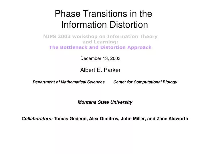
Phase Transitions in the Information Distortion. NIPS 2003 workshop on Information Theory and Learning: The Bottleneck and Distortion Approach December 13, 2003 Albert E. Parker. Department of Mathematical Sciences Center for Computational Biology Montana State University

E N D
Phase Transitions in the Information Distortion NIPS 2003 workshop on Information Theory and Learning: The Bottleneck and Distortion Approach December 13, 2003 Albert E. Parker Department of Mathematical Sciences Center for Computational Biology Montana State University Collaborators: Tomas Gedeon, Alex Dimitrov, John Miller, and Zane Aldworth
X Z q(Z|X) K objects N clusters The Goal: To determine the phase transitions or the bifurcation structure of solutions to clustering problems of the form maxqG(q) constrained byD(q)I0 where • is the set of valid conditional probabilities in RNK. • G and D are sufficiently smooth in . • G and D have symmetry: they are invariant to relabelling of the classes of Z. • The Hessians qG andq D are block diagonal.
X Z q(Z|X) K objects N clusters A similar formulation: Using the method Lagrange multipliers, the goal of determining the bifurcation structure of solutions of the optimization problem can be rephrased as finding the bifurcation structure of stationary points of the problem maxq(G(q)+D(q)) where • [0,). • is the set of valid conditional probabilities in RNK. • G and D are sufficiently smooth in . • G and D have symmetry: they are invariant to relabelling of the classes of Z. • The Hessian q(G+ D) is block diagonal,and satisfies a set of regularity conditions at bifurcation: (e.g. the kernel of each block is one dimensional)
How: Use the Symmetries By capitalizing on the symmetries of the cost functions, we have described the bifurcation structure of stationary points to problems of the form maxqG(q) constrained byD(q)I0 or maxq(G(q)+D(q)) where • [0,). • is the set of valid conditional probabilities in RNK. • G and D are sufficiently smooth in . • G and D have symmetry: they are invariant to relabelling of the classes of Z. • The Hessian q(G+ D) is block diagonal,and satisfies a set of regularity conditions at bifurcation: (e.g. the kernel is one dimensional)
Examplesoptimizing at a distortion level D(Y,Z) D0 • Rate Distortion Theory(Shannon 1950’s) Minimal Informative Compression • min I(X,Z) constrained by D(X,Z) D0 • Deterministic Annealing(Rose 1990’s) A Clustering Algorithm • max H(Z|X) constrained by D(X,Z) D0
Examplesoptimizing at a distortion level D(Y,Z) D0 • Rate Distortion Theory(Shannon 1950’s) Minimal Informative Compression • max -I(X,Z) constrained by D(X,Z) D0 • Deterministic Annealing(Rose 1998) A Clustering Algorithm • max H(Z|X) constrained by D(X,Z) D0 • I(X,Z)=H(Z) – H(Z|X)
Inputs and Outputs and Clustered Outputs Inputs Outputs Clustered Outputs X Z Y q(Z|X) p(X,Y) L objects {yi} N objects {zi} K objects {xi}
Inputs and Outputs and Clustered Outputs Inputs Outputs Clustered Outputs X Z Y q(Z|X) p(X,Y) L objects {yi} N objects {zi} K objects {xi}
Two methods which use an information distortion function to cluster • Information Bottleneck Method (Tishby, Pereira, Bialek 1999) • min I(X,Z) constrained by DI(X,Z) D0 • max –I(X,Z) + I(Y;Z) • Information Distortion Method(Dimitrov and Miller 2001) • max H(Z|X) constrained by DI(X,Z) D0 • max H(Z|X) + I(Y;Z)
Two methods which use an information distortion function to cluster • Information Bottleneck Method (Tishby, Pereira, Bialek 1999) • min I(X,Z) constrained by DI(X,Z) D0 • max –I(X,Z) + I(Y;Z) • Information Distortion Method(Dimitrov and Miller 2001) • max H(Z|X) constrained by DI(X,Z) D0 • max H(Z|X) + I(Y;Z) The Hessian is always singular … (-I(X,Z) is not strictly concave) The theory which follows does not apply
Two methods which use an information distortion function to cluster • Information Bottleneck Method (Tishby, Pereira, Bialek 1999) • min I(X,Z) constrained by DI(X,Z) D0 • max –I(X,Z) + I(Y;Z) • Information Distortion Method(Dimitrov and Miller 2001) • max H(Z|X) constrained by DI(X,Z) D0 • max H(Z|X) + I(Y;Z) The Hessian is always singular … (I(X,Z) is not strictly concave) The theory which follows does not apply H(Z|X) is strictly concave) The theory which follows does apply
A basic annealing algorithm to solve • maxq(G(q)+D(q)) • Let q0 be the maximizer of maxqG(q), and let 0=0. For k 0, let (qk , k)be a solution to maxqG(q) + D(q). Iterate the following steps until • K= max for some K. • Perform -step: Let k+1 =k + dk where dk>0 • The initial guess for qk+1 at k+1 is qk+1(0) = qk + for some small perturbation . • Optimization: solve maxq (G(q) + k+1 D(q)) to get the maximizer qk+1 , using initial guess qk+1(0) .
Application of the annealing method to the Information Distortion problem maxq (H(Z|X) + I(X;Z)) when p(X,Y) is defined by four gaussian blobs q(Z|X) X Z p(X,Y) Y X K=52 outputs L=52 inputs K=52 outputs N=4 clusteredoutputs Y, Inputs Z, ClusteredOutputs X, Outputs X, Outputs
Evolution of the optimal clustering: Observed Bifurcations for the Four Blob problem: We just saw the optimal clusterings q* at some *= max. What do the clusterings look like for < max?? I(Y,Z) bits
q* Observed Bifurcations for the 4 Blob Problem Conceptual Bifurcation Structure ?????? I(Y,Z) bits Why are there only 3 bifurcations observed? In general, are there only N-1 bifurcations? What kinds of bifurcations do we expect: pitchfork-like, transcritical, saddle-node, or some other type? How many bifurcating branches are there? What do the bifurcating branches look like? Are they 1st order phase transitions (subcritical) or 2nd order phase transitions (supercritical) ? What is the stability of the bifurcating branches? Is there always a bifurcating branch which contains solutions of the optimization problem? Are there bifurcations after all of the classes have resolved ?
Recall the Symmetries:To better understand the bifurcation structure, we capitalize on the symmetriesof the function G(q)+D(q) class 1 class 3 Z X q(Z|X) : a clustering N objects {zi} K objects {xi}
Recall the Symmetries:To better understand the bifurcation structure, we capitalize on the symmetriesof the function G(q)+D(q) class 3 class 1 Z X q(Z|X) : a clustering N objects {zi} K objects {xi}
A partial lattice of the maximal subgroups S2 x S2 of S4
Define a Gradient Flow • Goal: To determine the bifurcation structure of stationary points of • maxq (G(q) + D(q)) • Method: Study the equilibria of the of the flow • Equilibria of this system (in RNK+K ) are possible solutions of the optimization problem • The Jacobian q,L(q*,*) is symmetric, and so only bifurcations of equilibria can occur. • The first equilibrium is q*(0 = 0) 1/N. • If wTqF(q*,) w < 0for every wker J,then q*() is a maximizer of . • The first equilibrium is q*(0 = 0) 1/N.
q* Existence Theorems for Bifurcating Branches • Given a bifurcation at a point fixed by SN , • Equivariant Branching LemmaThe Smoller-Wasserman Theorem • (Vanderbauwhede and Cicogna 1980-1) (Smoller and Wasserman 1985-6) • There are N bifurcating branches, each which have symmetry SN-1. • There are N!/(2m!n!) bifurcating branches which havesymmetry Sm x Sn if N=m+n.
q* Existence Theorems for Bifurcating Branches • Given a bifurcation at a point fixed by SN-1 , • Equivariant Branching LemmaThe Smoller-Wasserman Theorem • (Vanderbauwhede and Cicogna 1980-1) (Smoller and Wasserman 1985-6) • There are N-1 bifurcating branches, each which have symmetry SN-2. • There are (N-1)!/(2m!n!) bifurcating branches which havesymmetry Sm x Sn if N-1=m+n.
Observed Bifurcation Structure Group Structure
The Equivariant Branching Lemma shows that the bifurcation structure contains the branches … Observed Bifurcation Structure q* Group Structure
The subgroups {S2x S2} give additional structure … Observed Bifurcation Structure q* Group Structure
The subgroups {S2x S2} give additional structure … Observed Bifurcation Structure q* Group Structure
Theorem: There are at exactly K bifurcations on the branch (q1/N , ) whenever G(q1/N)is nonsingular Observed Bifurcation Structure q* There are K=52 bifurcations on the first branch
A partial subgroup lattice for S4 and the corresponding bifurcating directions given by the Equivariant Branching Lemma
A partial subgroup lattice for S4 and the corresponding bifurcating directions corresponding to subgroups isomorphic to S2 x S2.
This theory enables us to answer the questions previously posed …
q* Observed Bifurcations for the 4 Blob Problem Conceptual Bifurcation Structure ?????? Why are there only 3 bifurcations observed? In general, are there only N-1 bifurcations? What kinds of bifurcations do we expect: pitchfork-like, transcritical, saddle-node, or some other type? How many bifurcating solutions are there? What do the bifurcating branches look like? Are they subcritical or supercritical ? What is the stability of the bifurcating branches? Is there always a bifurcating branch which contains solutions of the optimization problem? Are there bifurcations after all of the classes have resolved ?
q* Conceptual Bifurcation Structure Why are there only 3 bifurcations observed? In general, are there only N-1 bifurcations? There are N-1 symmetry breaking bifurcations from SMto SM-1 for M N. What kinds of bifurcations do we expect: pitchfork-like, transcritical, saddle-node, or some other type? How many bifurcating solutions are there? There are at least N from the first bifurcation, at leastN-1 from the next one, etc. What do the bifurcating branches look like? They are subcritical or supercritical depending on the sign of the bifurcation discriminator(q*,*,uk) . What is the stability of the bifurcating branches? Is there always a bifurcating branch which contains solutions of the optimization problem? No. Are there bifurcations after all of the classes have resolved ? Generically, no.
Continuation techniques numerically illustrate the theoryusing the Information Distortion
q* I(Y,Z) bits
q* Bifurcating branches with symmetry S2 x S2=<(12),(34)> I(Y,Z) bits
I(Y,Z) bits Additional structure!!
I(Y,Z) bits I(Y,Z) bits
q* A closer look … I(Y,Z) bits
q* Bifurcation from S4toS3… I(Y,Z) bits
The bifurcation from S4toS3 is subcritical … I(Y,Z) bits (the theory predicted this since the bifurcation discriminator (q1/4,*,u)<0)
What does this mean regarding solutions of the original problems? I(Y,Z) bits (4)RH(I0) =maxqH(Z|X) constrained byI(Y,Z) I0 (7) maxq(H(Z|X) + I(Y,Z))
Theorem: • dR/dI0 = -(I0) • d2R/dI02 = -d(I0)/dI0 (4)RH(I0) =maxqH(Z|X) constrained byI(Y,Z) I0 (7) maxq(H(Z|X) + I(Y,Z))