Download
1 / 32
320 likes | 385 Views
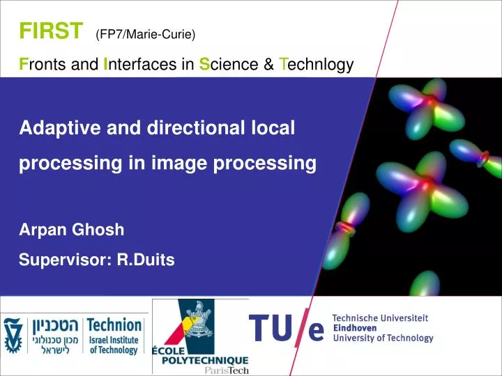
FIRST (FP7/ Marie-Curie ) F ronts and I nterfaces in S cience & T echnlogy Adaptive and directional local processing in image processing Arpan Ghosh Supervisor: R.Duits. Directional processing image processing. neural fibers in brain. bone-structure. catheters. muscle cells.

E N D
FIRST (FP7/Marie-Curie) Fronts and Interfaces in Science & Technlogy Adaptive and directional local processing in image processing ArpanGhosh Supervisor: R.Duits
Directional processing image processing neural fibers in brain bone-structure catheters muscle cells hart retinal bloodvessels Crack-Detection collagen fibres Challenge: Deal with crossings and fiber-context
Invertible Orientation Scores image kernel orientation score invertible
Extend to New Medical Image Modalities fibertracking fibertracking DTI HARDI Brownian motion of water molecules along fibers
Adaptive Left Invariant HJB-Equations on HARDI/DTI Input Viscosity solution
Challenges • The viscositysolutions of HJK are solvedby • morphologicalconvolution. Analytic/exact solutions ? • UseHJB-eqsforfiber tracking via Charpit’sequations • Canonicalequationson contact manifold ? • The left-invariantPDE’stake place alongautoparallels • w.r.t. Cartanconnection. SoNon-linearPDE’sby • best exp-curve fit to data ? • Exact solutions of geodesics
Problem considered currently • Let curve Curvature function • Corresponding energy functional • The challenge is to find for given end points and directions s.t.
The Setup • 5D manifold of positions & directions ℝ³×S² not a group! • Consider embedding of ℝ³×S² into the Lie group SE(3) ≔ ℝ³⋊SO(3) • By the quotient: ℝ³ ⋊ S² ≔ SE(3)/({0} ⋊SO(2)) • Consider Euler angle parameterization of S² for chart.
Differential Geometry Tools • SE(3) : Lie Group with group product • Unity element • Lie algebra
Left Invariant VF’s • A moving frame of reference using left invariant vector fields • The space of left invariant vector fields on SE(3) • Duals :
CommutatorTable • Lie brackets for the Lie algebra given by
Horizontal Curves in SE(3) • Curve is horizontal iff • Using the Frenet-Serret formulas, curvature and torsion of the spatial part of the curve are given by
Problem in the Moving Frame • The energy functional to minimize over all curves in SE(3): subject to the constraints along the curve :
15D Manifold • Consider the sub-Riemannian manifold • The constraints are 1 forms
Lagrangian 1-form on T*(Z): • Consider perturbations of stationary horizontal curves • Then, using Stoke’s theorem • For stationary curves, the above is 0 for all t. So,
Pfaffian System • By inserting 15 independent vectors from the sub-Riemannian manifold T(Z) and using Cartan’s structural formulas, we get
Solution for Curvature • The Pfaffian system produces the following
The Geodesics • Can get curve by solving Frenet frame equations • The last 6 equations from the system gives the equation for the geodesic where μ is a constant 6D row vector and m(g) is the 6×6 matrix representation of g∈ SE(3).
Transformed Curve • Choose s.t.
Boundary value problem • The boundary problem is solved by solving for 5 unknowns namely the following system • 6 dependent polynomial equations in the 5 variables above, of degree upto 8!
Current Focus • Solution of the boundary problem • Surjectivity of the geodesics • Study of the second variation of energy functional to prove optimality
Next target • Geometric fiber tracking based on the same Hamiltonian and Lagrangian framework with a cost coming from the enhanced data sets.