Download
1 / 21
210 likes | 317 Views
PSY 1950 Null Hypothesis Significance Testing September 29, 2008. vs. Finite Population Correction Factor. SEM and central limit theorem calculations are based on sampling with replacement from idealized, infinite populations

E N D
PSY 1950 Null Hypothesis Significance Testing September 29, 2008
Finite Population Correction Factor • SEM and central limit theorem calculations are based on sampling with replacement from idealized, infinite populations • Real-life research involves sampling without replacement from actual, finite populations • When n/N<.05, this doesn’t matter • When n/N>.05, use a correction factor:
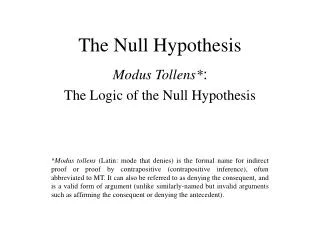
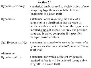
Controversy of NHST “backbone of psychological research” • Gerrig & Zimbardo (2002, p. 42) “a potent but sterile intellectual rake who leaves in his merry path a long train of ravished maidens but no viable scientific offspring” • Meehl (1967, p. 265) “…surely the most bone-headedly misguided procedure ever institutionalized in the rote training of science students” • Rozeboom (1997, p. 335)
NHST example (z-test) • State the null and alternative hypotheses • H0: µinfant = 26 lbs • H1: µ infant 26 lbs • Set the criteria for a decision • = .05 • |z| ≥ 1.96 • Collect data and compute sample statistics • Minfant = 30 lbs • with n = 16 and = 4 • z = (M - µ)/M = (30 - 26)/1 = 4 • Make a decision • Reject H0
NHST Errors Type III error?
Power • The probability of correctly rejecting a false null hypothesis = 1 - • http://wise.cgu.edu/power/power_applet.html
= .05 • “It is convenient to take this point as a limit in judging whether a deviation is to be considered significant or not. Deviations exceeding twice the standard deviation are thus formally regard as significant” • Fisher (1925, p. 47) • Historical roots prior to Fisher’s definition • Corresponds to subjective demarcation of chance from non-chance events • "... surely, God loves the .06 nearly as much as the .05” • (Rosnow & Rosenthal, 1989)
NHST Rationale • Why try to reject null hypothesis? • Philosophical: Popperian falsifiability • accept H1: the projector occasionally malfunctions • reject H0: the projector always works • Practical: defining the sampling distribution • H1: the projector failure rate = ? • H0: the projector failure rate = 0%
History of NHST Fisher’s (1925) NHST: • Set up null hypothesis (not necessarily) • Report exact significance • Only do this when you know little else Neyman & Pearson (1950) • Set up two competing hypothesis, H1 and H2, and make a priori decisions about and • If data falls into rejection region of H1, accept H2; otherwise accept H1. Acceptance belief. • Only do this when you have a disjunction of hypotheses (either H1 or H2 is true) Current NHST (according to some): • Set up null hypothesis as nil hypothesis • Reject null at p<.05 and accept your hypothesis • Always do this
Criticisms of NHST • Affirming the consequent • If P then Q. Q. Therefore P. • The straw person argument • Tukey (1991): “It is foolish to ask ‘Are the effects of A and B different?’ They are always different—for some decimal place”(p. 100) • “Statistical significance does not necessarily imply practical significance!” • The replication fallacy • If you conduct an experiment that results in p = .05 (two-tailed), what is the chance that a replication of that experiment will produce a statistically significant (p<.05) effect? • 50% (see Cumming, 2008, Appendix B) • “Confusion of the inverse” • “absence of proof is not proof of absence” • “presence of proof is not proof of presence”
Affirming the Consequent • NHST commits logical fallacy • NHST: If the null hypothesis is correct, then these data are highly unlikely • These data have occurred • Therefore, the null hypothesis is highly unlikely • Analog: If a person is an American, then he is probably not a member of Congress • This person is a member of Congress • Therefore, he is probably not an American • Response: Science progresses through testing its predictions • Logic may be flawed, but success is hard to deny
The Straw Person Argument • Often null hypothesis = nil hypothesis • The nil hypothesis is always (or almost always) false • The “crud factor” in correlational research (Meehl, 1990) • The “princess and the pea” effect in experimental research • If the null hypothesis is always false, how does rejecting it increase knowledge? • Response: effect size matters, statistical significance is not practical significance, test interactions
Replication Fallacy • p-values don’t say much about replicability, yet most everyone thinks they do • Replication is NOT 1 - (Tversky & Kahneman, 1971) • Response: p-values inform replicability, just less than one might think • All else equal, the lower the p-value, the higher the replicability
“Confusion of the Inverse” • Criticism: NHST calculates the probability of obtaining the data given a hypothesis, p(D|H0), not the probability of obtaining a hypothesis given the data, p(H0|D) • A p-value of .05 does NOT necessarily indicate that the null hypothesis is unlikely to be true • Response: logically faulty but productive inferences is better than nothing • p(D|H0) approximates p(H0|D) under typical experimental settings where p(H0) is low, i.e., p(H1) > p(H0) • p(H0|D) varies monotonically with p(D|H0) p(H0|D) • When p(H0) = .35, p(H0|D) = .35 • p(D|H0) and p(H0|D) are correlated (r = .38)
Reconciliation • “Inductive inference cannot be logically justified, but they can be defended pragmatically” (Krueger, 2001) • Use NHST mindfully • “There is no God-given rule about when and how to make up your mind in general.” • Hays (1973, p. 353) • Don’t rely exclusively on p-values
Alternatives to p-values • Effect size • Meta-analysis • Confidence intervals • prep