Download
1 / 48
960 likes | 1.92k Views
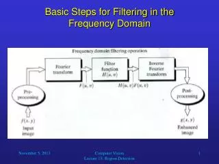
Digital Image Processing. Filtering in the Frequency Domain (Circulant Matrices and Convolution). Christophoros Nikou cnikou@cs.uoi.gr. Toeplitz matrices. Elements with constant value along the main diagonal and sub-diagonals.

E N D
Digital Image Processing Filtering in the Frequency Domain (Circulant Matrices and Convolution) ChristophorosNikou cnikou@cs.uoi.gr
Toeplitz matrices • Elements with constant value along the main diagonal and sub-diagonals. • For a NxN matrix, its elements are determined by a (2N-1)-length sequence
Toeplitz matrices (cont.) • Each row (column) is generated by a shift of the previous row (column). • The last element disappears. • A new element appears.
Circulant matrices • Elements with constant value along the main diagonal and sub-diagonals. • For a NxN matrix, its elements are determined by a N-length sequence
Circulant matrices (cont.) • Special case of a Toeplitz matrix. • Each row (column) is generated by a circularshift (modulo N) of the previous row (column).
Convolution by matrix-vector operations • 1-D linear convolution between two discrete signals may be expressed as the product of a Toeplitz matrix constructed by the elements of one of the signals and a vector constructed by the elements of the other signal. • 1-D circular convolution between two discrete signals may be expressed as the product of a circulant matrix constructed by the elements of one of the signals and a vector constructed by the elements of the other signal. • Extension to 2D signals.
1D linear convolution using Toeplitz matrices • The linear convolution g[n]=f [n]*h [n] will be of length N=N1+N2-1=3+2-1=4. • We create a Toeplitz matrix H from the elements of h [n] (zero-padded if needed) with • N=4 lines (the length of the result). • N1=3 columns (the length of f [n]). • The two signals may be interchanged.
1D linear convolution using Toeplitz matrices (cont.) Length of the result =4 Notice that H is not circulant (e.g. a -1 appears in the second line which is not present in the first line. Length of f [n] = 3 Zero-padded h[n] in the first column
1D circular convolution using circulant matrices • The circular convolution g[n]=f [n]h [n] will be of length N=max{N1, N2}=3. • We create a circulant matrix H from the elements of h [n] (zero-padded if needed) of size NxN. • The two signals may be interchanged.
1D circular convolution using circulant matrices (cont.) Zero-padded h[n] in the first column
Block matrices • Aij are matrices. • If the structure of A, with respect to its sub-matrices, is Toeplitz (circulant) then matrix A is called block-Toeplitz(block-circulant). • If each individual Aij is also a Toeplitz (circulant) matrix then A is called doubly block-Toeplitz(doubly block-circulant).
2D linear convolution using doubly block Toeplitz matrices m m 1 1 1 4 1 1 -1 2 5 3 n n h [m,n] f [m,n] M1=2, N1=3 M2=2, N2=2 The result will be of size (M1+M2-1) x (N1+N2-1) = 3 x 4
2D linear convolution using doubly block Toeplitz matrices (cont.) m m 1 1 1 4 1 1 -1 2 5 3 n n h [m,n] f [m,n] • At first, h[m,n] is zero-padded to 3 x 4 (the size of the result). • Then, for each row ofh[m,n], a Toeplitz matrix with 3 columns (the number of columns of f [m,n]) is constructed. m 0 0 0 0 1 1 0 0 0 1 -1 0 n h[m,n]
2D linear convolution using doubly block Toeplitz matrices (cont.) • For each row ofh[m,n], a Toeplitz matrix with 3 columns (the number of columns of f [m,n]) is constructed. m 0 0 0 0 1 1 0 0 0 1 -1 0 n h[m,n]
2D linear convolution using doubly block Toeplitz matrices (cont.) m m 1 1 1 4 1 1 -1 2 5 3 n n h [m,n] f [m,n] • Using matrices H1, H2and H3 as elements, a doubly block Toeplitz matrix H is then constructed with 2 columns (the number of rows of f [m,n]).
2D linear convolution using doubly block Toeplitz matrices (cont.) m m 1 1 1 4 1 1 -1 2 5 3 n n h [m,n] f [m,n] • We now construct a vector from the elements of f [m,n].
2D linear convolution using doubly block Toeplitz matrices (cont.) m m 1 1 1 4 1 1 -1 2 5 3 n n h [m,n] f [m,n]
2D linear convolution using doubly block Toeplitz matrices (cont.)
2D linear convolution using doubly block Toeplitz matrices (cont.) m m m 1 1 3 1 10 4 1 5 * 1 -1 2 2 5 3 -2 3 n n n h [m,n] g [m,n] f [m,n] 1 5 5 1 = 2 3
2D linear convolution using doubly block Toeplitz matrices (cont.) Another example m m 3 4 1 -1 1 2 n n h [m,n] f [m,n] M1=2, N1=2 M2=1, N2=2 The result will be of size (M1+M2-1) x (N1+N2-1) = 2 x 3
2D linear convolution using doubly block Toeplitz matrices (cont.) m m 3 4 1 -1 1 2 n n h [m,n] f [m,n] • At first, h[m,n] is zero-padded to 2 x 3 (the size of the result). • Then, for each line ofh[m,n], a Toeplitz matrix with 2 columns (the number of columns of f [m,n]) is constructed. m 0 0 0 1 -1 0 n h[m,n]
2D linear convolution using doubly block Toeplitz matrices (cont.) • For each row ofh[m,n], a Toeplitz matrix with 2 columns (the number of columns of f [m,n]) is constructed. m 0 0 0 1 -1 0 n h[m,n]
2D linear convolution using doubly block Toeplitz matrices (cont.) m m 3 4 1 -1 1 2 n n h [m,n] f [m,n] • Using matrices H1and H2 as elements, a doubly block Toeplitz matrix H is then constructed with 2 columns (the number of rows of f [m,n]).
2D linear convolution using doubly block Toeplitz matrices (cont.) m m 3 4 1 -1 1 2 n n h [m,n] f [m,n] • We now construct a vector from the elements of f [m,n].
2D linear convolution using doubly block Toeplitz matrices (cont.) m m 3 4 1 -1 1 2 n n h [m,n] f [m,n]
2D linear convolution using doubly block Toeplitz matrices (cont.)
2D linear convolution using doubly block Toeplitz matrices (cont.) m m m 3 1 4 * 3 4 1 1 -2 n 1 -1 1 2 n n g [m,n] h [m,n] f [m,n] =
2D circular convolution using doubly block circulant matrices The circular convolution g[m,n]=f [m,n]h [m,n] with may be expressed in matrix-vector form as: where H is a doubly block circulant matrix generated by h [m,n]and f is a vectorized form of f [m,n].
2D circular convolution using doubly block circulant matrices (cont.) Each Hj, forj=1,..M, is a circulant matrix with N columns (the number of columns of f [m,n]) generated from the elements of the j-throw of h [m,n].
2D circular convolution using doubly block circulant matrices (cont.) Each Hj, forj=1,..M, is a NxNcirculant matrix generated from the elements of the j-throw of h [m,n].
2D circular convolution using doubly block circulant matrices (cont.) m m 0 0 0 0 1 0 0 0 1 1 3 -1 0 1 -1 1 1 2 n n h [m,n] f [m,n]
2D circular convolution using doubly block circulant matrices (cont.) m m 0 0 0 0 1 0 0 0 1 1 3 -1 0 1 -1 1 1 2 n n h [m,n] f [m,n]
2D circular convolution using doubly block circulant matrices (cont.)
2D circular convolution using doubly block circulant matrices (cont.) m m m 0 0 0 0 1 4 1 -2 0 0 0 1 3 1 4 3 -1 -3 0 1 -1 -1 1 0 1 2 2 n n n h [m,n] f [m,n] g [m,n] =
Diagonalization of circulant matrices Theorem: The columns of the inverse DFT matrix are eigenvectors of any circulant matrix. The corresponding eigenvalues are the DFT values of the signal generating the circulant matrix. Proof: Let be the DFT basis elements of length N with:
Diagonalization of circulant matrices (cont.) We know that the DFT F [k] of a 1D signal f [n] may be expressed in matrix-vector form: where
Diagonalization of circulant matrices (cont.) The inverse DFT is then expressed by: where The theorem implies that any circulant matrix has eigenvectors the columns of A-1.
Diagonalization of circulant matrices (cont.) Let H be a NxNcirculant matrix generated by the 1D N-length signal h[n], that is: Let also αk be the k-th column of the inverse DFT matrix A-1. We will prove that αk, for any k, is an eigenvector of H. The m-th element of the vector Hαk, denoted by is the result of the circular convolution of the signal h[n]with αk.
Diagonalization of circulant matrices (cont.) We will break it into two parts
Diagonalization of circulant matrices (cont.) Periodic with respect to N.
Diagonalization of circulant matrices (cont.) DFT of h[n] at k. This holds for any value of m. Therefore: which means thatαk, for any k, is an eigenvector of H with corresponding eigenvalue the k-th element of H[k], the DFT of the signal generating H.
Diagonalization of circulant matrices (cont.) The above expression may be written in terms of the inverse DFT matrix: or equivalently: Based on this diagonalization, we can prove the property between circular convolution and DFT.
Diagonalization of circulant matrices (cont.) DFT of g[n] DFT of h [n] DFT of f [n]
Diagonalization of doubly block circulant matrices • These properties may be generalized in 2D. • We need to define the Kronecker product:
Diagonalization of doubly block circulant matrices (cont.) • The 2D signal f [m,n], • may be vectorized in lexicographic ordering (stacking one column after the other) to a vector: • The DFT of f [m,n], may be obtained in matrix-vector form:
Diagonalization of doubly block circulant matrices (cont.) Theorem: The columns of the inverse 2D DFT matrix are eigenvectors of any doubly block circulant matrix. The corresponding eigenvalues are the 2D DFT values of the 2D signal generating the doubly block circulant matrix: Diagonal, containing the 2D DFT of h[m,n] generating H Doubly block circulant