Download

1 / 17
170 likes | 329 Views
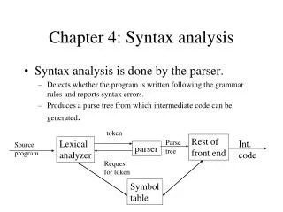
Chapter 4. Syntax Analysis (1). Application of a production A in a derivation step i i+ 1. Formal grammars (1/3). Example : Let G 1 have N = { A , B , C }, T = { a , b , c } and the set of productions A CB BC A aABC bB bb

E N D
Application of a production A in a derivation step i i+1
Formal grammars (1/3) • Example : Let G1have N = {A, B, C}, T = {a, b, c} and the set of productions A CB BC A aABC bB bb A abC bC bc cC cc The reader should convince himself that the word akbkck is in L(G1) for all k 1 and that only these words are in L(G1). That is, L(G1) = { akbkck | k 1}.
Formal grammars (2/3) • Example : Grammar G2is a modification of G1: G2: A CB BC A aABC bB bb A abC bC b The reader may verify that L(G2) = { akbk | k 1}. Note that the last rule, bC b, erases all the C's from the derivation, and that only this production removes the nonterminal C from sentential forms.
Formal grammars (3/3) • Example : A simpler grammar that generates { akbk | k 1} is the grammar G3: G3: S S aSb S ab A derivation of a3b3 is S aSb aaSbb aaabbb The reader may verify that L(G3) = { akbk | k 1}.
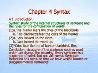
Contracting Noncon- tracting Regular The four types of formal grammars
Context-Sensitive Grammars(Type1) Unrestricted Grammars(Type0) • Definition : A context-sensitive grammarG = (N,T,P,) is a formal grammar in which all productions are of the form φAψ→φωψ, ω≠ The grammar may also contain the production →, if G is a context-sensitive (type1) grammar, then L(G) is a context-sensitive (type1) language.
Context-Free Grammars (Type2) • Definition : A context-free grammarG=(N,T,P,) is a formal grammar in which all productions are of the form A→ω The grammar may also contain the production →λ. If G is a context-free (type2) grammar, then L(G) is a context-free (type2) language. A∈N∪{} ω∈(N∪T)*-{λ}
Regular Grammars (Type3) (1/2) • Definition : A production of the form A→aB or A→a is called a right linear production. A production of the form A→Ba or A→a is a left linear production. A formal grammar is right linear if it contains only right linear productions, and is left linear if it contains only left linear production →λ. Left and right linear grammars are also known as regular grammars. If G is a regular (type3) grammar, then L(G) is a regular (type3) language. A∈N∪{∑} B∈N a∈T A∈N∪{∑} B∈N a∈T
Regular Grammars (Type3) (2/2) • Example: A left linear grammar G1 and a right linear grammar G2 have productions as follows: G1 : G2: The reader may verify that L(G1) = (10)*1=1(01)*=L(G2) ∑ → 1B ∑ → 1 A → 1B B → 0A A → 1 ∑ → B1 ∑ → 1 A → B1 B → A0 A → 1
Operator-Precedence Relations from Associativity and Precedence (1/2) 1. If operator θ1 has higher precedence than operator θ2, make θ1 ·> θ2 and θ2 <· θ1 . For example, if * has higher precedence than +, make * ·> + and + <· *. These relations ensure that, in an expression of the form E+E*E+E, the central E*E is the handle that will be reduced first. 2. If θ1 and θ2 are operators of equal precedence (they may in fact be the same operator), then make θ1 ·> θ2 and θ2 ·> θ1 if the operators are left-associative, or make θ1 <· θ2 and θ2 <· θ1 if they are right-associative. For example, if + and – are left-associative, then make + ·> +, + ·> -, - ·> - and - ·> +. If is right associative, then make <· . These relations ensure that E-E+E will have handle E-E selected and EEE will have the last EE selected.
Operator-Precedence Relations from Associativity and Precedence (2/2) 3. Make θ <· id, id ·> θ, θ <· (, ( <· θ , ) ·> θ, θ ·> ), θ ·> $, and $ <· θ for all operators θ. Also, let These rules ensure that both id and (E) will be reduced to E. Also, $ serves as both the left and right endmarker, causing handles to be found between $’s wherever possible. ·
· Fig. 4.25. Operator-precedence relations.
Precedence Functions Example 4.29 The Precedence table of Fig. 4.25 has the following pair of precedence functions, For example, * <·id and, f(*) < g(id). Note that f(id) > g(id) suggests that id·> id; but, in fact, no precedence relation holds between id and id. Other error entries in Fig. 4.25 are similarly replaced by one or another precedence relation.