Download
1 / 24
240 likes | 365 Views
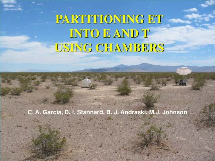
PARTITIONING ET INTO E AND T USING CHAMBERS. C. A. Garcia, D. I. Stannard, B. J. Andraski, M.J. Johnson. OUTLINE. Importance in hydrologic studies Discrete measurements of E and T Component-scale fluxes Landscape-scale fluxes Comparisons with eddy-covariance ET

E N D
PARTITIONING ET INTO E AND T USING CHAMBERS C. A. Garcia, D. I. Stannard, B. J. Andraski, M.J. Johnson
OUTLINE • Importance in hydrologic studies • Discrete measurements of E and T • Component-scale fluxes • Landscape-scale fluxes • Comparisons with eddy-covariance ET • Continuous estimates of E and T
IMPORTANCE OF CHAMBERS IN HYDROLOGIC STUDIES • Limited Fetch • Determine factors controlling ET • Heterogeneous settings • Soil-plant-atmosphere interactions • Spatial variability of ET fluxes • Determine contaminant fluxes to atmosphere • Determine relative rates of water use
Limited Fetch Bare soil over a leach field Turf Grass at a city park
DISCRETE MEASUREMENTS • Component- and landscape-scale estimates • Two Case Studies • Amargosa Desert Research Site (ADRS) • Arid site in southern Nevada • Measurements of plants and bare soil made quarterly (August 2003–January 2006) • Walnut Gulch (WG), Arizona • Semi-arid site in southeastern Arizona • Three days of plant and bare-soil measurement (August 1, 8, and 9, 1990)
Slope of Vapor Density Curve Slope computed using a 5–10 point regression
One-Layer, Multi-Component Model Component-scale λE Component-scale λT (Stannard, 1988) λETls – landscape-scale latent heat flux in W/m2 Fc – fractional cover of plant species (i) or bare soil (s) λETi – chamber latent-heat flux in W/m2, combined plant and soil Rc – relative crown cover λETs – chamber latent-heat flux in W/m2, bare soil only
ADRS Two perpendicular 400-m transects 4 measured species 6–10% plant cover Dominant species is 80% of plant cover WG Five parallel 30.5-m transects 5 measured species 26% plant cover Dominant species is 40% of plant cover Fractional Cover of Plants and Bare Soil
Relative Crown Cover • Rc ranges from • 20 – 70% cover at ADRS • 15 – 40% cover at WG (Stannard, 1988) Rc – relative crown cover H – camera height h – major axis of plant crown Rc’ – ratio of plant crown cover to chamber area
Discrete Component-Scale Fluxes • Bare soil fluxes were lowest as a result of drier surface soils • ADRS vegetation • Wolfberry was greatest in spring • Creosote bush was greatest during the summer, fall, and winter • WG vegetation • Desert zinnia and tarbush fluxes were greatest • Upper canopy negatively correlated with shallow soil-water content • Lower canopy correlated with air temperature and relative humidity • Leaves closer to the ground undergo greater temperature changes • Saturation-vapor pressure increases with increasing temperature
Discrete Landscape-Scale Fluxes • Bare-soil importance substantially increased as a result of Fc • ADRS – soil contribution was greater than each plant • WG – soil contribution was greater than 4 of 5 plants • E and T partitioning • ADRS – 60% E to 40% T on 5/2/2005; – 70%E to 30% T over all periods • WG – 15% E to 85% T over three days measured
Landscape-scale ETChamber vs. EC • ADRS • Over all periods, chamber ET was 7% less than EC • No clear trend relating chamber ET to EC ET • Temperature • Antecedent moisture • Season • WG • Over 3 days, chamber ET ~30% greater than EC • Difference likely due to high bias in chamber ET • Mismatch of internal air and external wind speed • Chamber heating during measurement
CONTINUOUS ET ESTIMATES Partitioning continuous ET into E and T • Continuous • ET: measured (eddy-covariance station) • E: estimated (Priestley-Taylor Model) • Periodic chamber measurements from bare soil • Continuous micrometeorological data • Soil water content • Net radiation • Ground heat flux • Air temperature • T: estimated from daily ET − E
Priestley-Taylor Model (Modified by Davies and Allen, 1973) α′ = f(θ), 0 < θ < θns α′= 1.26, θ≥ θns λE – actual latent heat flux, W/m2 α’ – Priestley-Taylor coefficient S – slope of saturation vapor pressure temperature curve, g/m3/K γ – psychrometric constant Rn –net radiation, W/m2 G – ground heat flux, W/m2
Priestley-Taylor Calibration Dataset follows a linear, segmented model α’ = 5.07 θ – 0.03, 0 < θ < θns α’ = 1.26, θ≥ θns
Continuous ET Partitioned into E and T 75%E to 25%T
ET PartitioningPriestley-Taylor Approach vs. Lysimeters • Weighing lysimeters commonly used as direct measure of water balance • Measure ET from vegetated lysimeter • Measure E from bare soil lysimeter (devoid of roots)
Lysimeter Case Study at the Nevada Test Site (NTS) E-to-T partitioning at NTS was within 10–15 percent 75% E to 25% T 85% E to 15% T
Lysimeter Case Study • Major difference in partitioning was experimental design • ADRS – E measured from plant-interspace areas • NTS – E measured from bare soil devoid of roots • In Mojave Desert • Shrub roots extend laterally up to 4 m • Soil-water extraction beneath canopies is similar to interspace areas
CONCLUSIONS • Chambers help quantify contributions to ET in mixed communities • Chamber estimates of landscape-scale ET • ADRS – 7% less than eddy-covariance ET • WG – 30% greater than eddy-covariance ET • ET partitioning into E and T • ADRS – 70% E to 30% T (discrete) and 75% E to 25% T (cont.) • WG 15% E to 85% T • ADRS - ongoing numerical modeling shows 72%E to 28%T for cumulative ET