Download
1 / 52
520 likes | 631 Views
Sensor Networks From The Network Perspective. Anxiao (Andrew) Jiang. Paradise Mini-Workshop. 05/18/2006. Berkeley/SF. Examples of Sensor Network Applications. Microclimate monitoring of redwood forest (UC Berkeley). 70% of H2O cycle is through trees, not ground

E N D
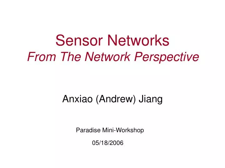
Sensor Networks From The Network Perspective Anxiao (Andrew) Jiang Paradise Mini-Workshop 05/18/2006
Berkeley/SF Examples of Sensor Network Applications Microclimate monitoring of redwood forest (UC Berkeley) • 70% of H2O cycle is through trees, not ground • Complex interactions of tree growth and environment • Need to understand dynamic processes within the trees
Examples of Sensor Network Applications Microclimate monitoring of redwood forest (UC Berkeley) Ad Hoc Multihop Network
Acadia National Park Mt. Desert Island, ME Great Duck Island Nature Conservancy Burrowmote and petrel Examples of Sensor Network Applications Habitat Monitoring on Great Duck Island (UC Berkeley)
Internet Examples of Sensor Network Applications Habitat Monitoring on Great Duck Island (UC Berkeley) Patch Network Sensor Node Sensor Patch Gateway Transit Network Client Data Browsing and Processing Basestation Base-Remote Link Data Service
Examples of Sensor Network Applications Habitat Monitoring on Great Duck Island (UC Berkeley)
battery Examples of Sensors • Light Sensors • Environmental Sensors • humidity + temp • Pressure + temp WeatherMote antenna Functions of a sensor: mote Collecting data Computation Communication
Examples of Sensors MICA mote
Properties of Sensor Networks Sensing, computation, communication Ad hoc, self-configuration Long lived, large, unattended In network processing, save energy Asks for adaptive and fault tolerant algorithms
Implications: Computation Computation with limited memory, limited energy, locality Distributed computing, peer to peer, collaborative Collective behavior Noisy measurements, dynamic conditions, failures Data collection, aggregation, computation, communication
Implications: Networking New networks, new properties, new interfaces
Implications: Networking An example of sensornet architecture David Culler, et al., UC Berkeley
“Small” Technology, Broad Agenda (Culler, 2005) • Social factors • security, privacy, information sharing • Applications • long lived, self-maintaining, dense instrumentation of previously unobservable phenomena • interacting with a computational environment • Programming the Ensemble • describe global behavior, synthesis local rules that have correct, predictable global behavior • Distributed services • localization, time synchronization, resilient aggregation • Networking • self-organizing multihop, resilient, energy efficient routing • despite limited storage and tremendous noise • Operating system • extensive resource-constrained concurrency, modularity • framework for defining boundaries • Architecture • rich interfaces and simple primitives allowing cross-layer optimization • Components • low-power processor, ADC, radio, communication, encryption, sensors, batteries
Routing Routing in General Networks Shortest path routing Compact routing: smaller routing tables, bounded stretch factor Hierarchical routing: BGP, OSPF Large sensor networks: We can use geographic locations.
Routing Greedy Forwarding Assumptions: source Every node knows its location and its neighbors’ locations The source knows the location of the destination Greedy Forwarding: A node always forwards the message to a neighbor whose Euclidean distance to the destination is smaller. destination
Routing Greedy Forwarding Can Fail destination When the message reaches node x, no next hop can be selected for Greedy Forwarding, because both w and y are further away from D than x is.
Routing: Face Routing Planarization of a graph: Mark some edges as unusable, so that the remaining graph is a connected planar graph.
Routing: Face Routing If the graph is a unit disk graph (UDG), there are localized ways to planarize it: Gabriel Graph: Restricted Delaunay Graph: Relative Neighborhood Graph:
Routing: Face Routing Face routing is nearly stateless. (Nearly) no routing tables. face face face face face source destination GFG: [Bose01] GPSR (Greedy Perimeter Stateless Routing): [Karp00]
Routing: Virtual Coordinates When node locations are unknown, we can do embedding. Rubber-band algorithm for embedding Geographic Routing without Location Information, Rao et al., MobiCom’03
Routing: Virtual Coordinates Rubber-band algorithm for embedding Perimeter nodes do not change their coordinates. Non-perimeter nodes update their coordinates through multiple iterations. In each iteration, it takes its coordinates as the average coordinates of its neighbors.
Routing: Virtual Coordinates in 3-D Idea: Embed the network in a high-dimensional space, and/or define new ways of ‘greedy forwarding.’ Theorem: Any graph containing a 3-connected planar spanning sub-graph can be embedde in the 3-dimensional Euclidean space, where greedy forwarding guarantees delivery using a new distance function. On A Conjecture Related to Geometric Routing, Papadimitriou et al., manuscript.
Routing: Location Free Routing Use geometric properties, not node locations. New naming and routing system for nodes. GLIDER Fang, Gao, Guibas, de Silva, Zhang, GLIDER: Gradient Landmark-based Distributed Routing for Sensor Networks, INFOCOM 2005.
Routing: Location Free Routing Use geometric properties, not node locations. New naming and routing system for nodes. MAP Blue: MAP Green: GPSR (geographical forwarding) Bruck, Gao, Jiang, MAP: Medial Axis Based Geometric Routing In Sensor Networks, MobiCom 2005.
Network Localization Definition: Determine the (relative) positions of nodes based on known information. Location information that can be learned in a wireless network: Connectivity Sometimes, also … Distance between adjacent nodes Angle between adjacent edges Knowing the locations of nodes are important for: The meaning of data Routing Tasking
Network Localization Note: truthful localization is not always feasible … A most simple example where truthful localization is not feasible: Known information: there are three nodes A, B, C; A and B are adjacent; B and C are adjacent. We cannot tell which of the following localizations is true. All are possible … C C A B C A B A B For a large network, generally, valid localizations (localizations that conform to the known information) are similar to the truthful localization. So we are interested in finding just one valid localization. Valid localization: localization that conform to the known information.
Network Localization Hardness of Localization Network model: Unit disk graph model. Hardness results: No good known approximation algorithm.
Network Localization Practical Techniques: Trilateration, triangulation, multileration …
Network Localization Practical Techniques: Mass-Spring Method Edges are springs, whose lengths equal their measured distance. Multidimensional Scaling (MDS) Given the estimated distance matrix, take the largest d eigenvalues and eigenvectors of the distance matrix to get the d-dimensional approximate embedding. More: Dynamic algorithms, robust to errors …
Detect Important Geometric Features Hole Detection Topological Hole Detection in Wireless Sensor Networks and Its Applications, Funke, DIALM-POMC’05.
Detect Important Geometric Features Hole Detection (for Quasi-UDG model) Kroller, Fekete, Pfisterer, Fischer, Deterministic boundary recognition and topology extraction for large sensor networks, SODA 2006.
Detect Important Geometric Features Cut Detection (For linear cut only) Shrivastava, Suri and Toth, Detecting cuts in sensor networks, ISPN 2005.
Location Service Basic Scenario: Node A needs to send messages to node B via location-based routing. Node A only knows node B’s ID, not its location. What can we do? We need Location Service to make it work.
Location Service Scenario: Node A needs to send messages to node B via location-based routing. Node A only knows node B’s ID, not its location. Solution: Node B has a location server, whose position is common known to all nodes. Node B sends its location to that server. Node A retrieves node B’s location from that server. A B B’s location server
Location Service GLS --- a distributed geographic location service Properties of GLS: Decentralized. There is no special node in the network; no infrastructure is needed. Each node acts as a location server for a small number of other nodes. Scalable. It enables construction of network that scales to a large number of nodes. Fault-tolerant. There is no dependence on specially designated nodes. When network is partitioned, it operates effectively in each network component. Locality-sensitive: when querying the location of a nearby node, the query path is short. Reference: A Scalable Location Service for Geographic Ad Hoc Routing, by Li, Jannotti, De Couto, Karger, Morris, MobiCom’00
Location Service GLS --- a distributed geographic location service For each square that node u is in and its three sibling squares, u will have a location server. Update: Send a node’s location to its servers. Query: Find a nearby location server of the destination node. Use Consistent Hashing to reduce the size of routing tables.
Data Centric Storage Data-centric storage: Sensed data are stored at a node determined by the name associated with the sensed data. GHT: A Geographic Hash Table for Data-Centric Storage, Ratnasamy et al., 2002. Basic elements in GHT: GHT hashes keys into geographic coordinates, and stores a key-value pair at the sensor node geographically nearest the hash of its key.
Data Centric Storage GHT: Geographic Hash Table Basic elements in GHT: Hash(elephant sighting)=(23,36) Key: elephant sighting 23,36 Key: elephant sighting Value: # of elephants: one Time: 9:02am Location: xxxx sensornet The system replicates stored data locally to ensure persistence when nodes fail.
Multi-Resolution Storage Ganesan, Greenstein, Perelyubskiy, Estrin and Heidemann, An evalution of multi-resolution Storage for sensor networks, SenSys 2003.
Directed Diffusion: Query by Interest Dissemination Basic process of directed diffusion: Users spread their interests for data in the network; the interests received by a node pull the related data toward it; good routing paths are reenforced over time. Directed Diffusion: A Scalable and Robust Communication Paradigm for Sensor Networks, Intanagonwiwat, Govindan, Estrin, MobiCom’00.
Query of Sensor Networks Aggregation Sensor applications depend on the ability to extract data from the network. Often, the data consists of aggregations (or summaries) rather than raw sensor readings. Examples of data aggregates: MAX MEDIAN MIN COUNT DISTINCT HISTOGRAM COUNT SUM AVERAGE
Query of Sensor Networks Aggregate data in a tree(Implemented in TinyDB project at Berkeley and Cougar project at Cornell) users inject queries basestation (resource rich)
Query of Sensor Networks Aggregate data in a tree(Implemented in TinyDB project at Berkeley and Cougar project at Cornell) users inject queries basestation (resource rich)
Query of Sensor Networks Aggregate data in a tree(Implemented in TinyDB project at Berkeley and Cougar project at Cornell) users inject query: MAX basestation (resource rich) 8 19 12 10 4 8 11 27 2 7 12 6 5 1 12 3 10 9 local data
Query of Sensor Networks Aggregate data in a tree(Implemented in TinyDB project at Berkeley and Cougar project at Cornell) users inject query: MAX 27 basestation (resource rich) 19 27 8 8 19 12 27 12 8 10 10 12 4 27 8 12 12 11 10 27 2 9 7 1 12 12 6 3 5 10 9 1 12 3 10 9 local data
Query of Sensor Networks Aggregation: Data Structures for More Complex Queries • Use Q-Digest to Support Aggregation Queries • Quantile query • i-thvalue • Reverse quantile query • Value i-th • Consensus query • Most frequent? • Histogram Medians and Beyond: New Aggregation Techniques for Sensor Networks, Shrivastava et al., SenSys’04.
Query of Sensor Networks Aggregation: Data Structures for More Complex Queries Example of Q-Digest:
Query of Sensor Networks More: Massive data, distributed, noisy measurement, errors, complex queries, historical data, real time data, streaming algorithms, dynamic update, privacy ……
Sensing Coverage and Exposure Coverage / Exposure: Sensors observe targets. Observe a single target, multiple targets, or a sensor field. From the target’s point of view Exposure. From the sensor’s point of view Coverage. Minimize / maximize exposure, maximize coverage.