Download
1 / 16
170 likes | 181 Views
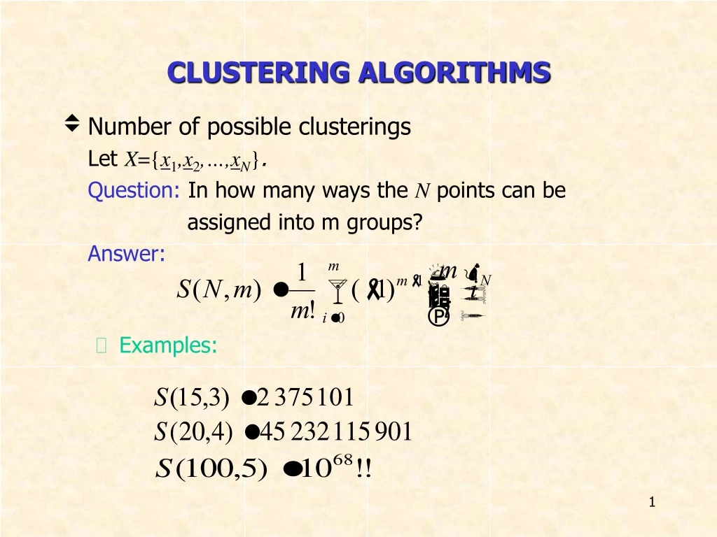
CLUSTERING ALGORITHMS. Number of possible clusterings Let X ={ x 1 , x 2 ,…, x N } . Question: In how many ways the N points can be assigned into m groups? Answer: Examples :. A way out:

E N D
CLUSTERING ALGORITHMS • Number of possible clusterings Let X={x1,x2,…,xN}. Question:In how many ways the N points can be assigned into m groups? Answer: • Examples:
A way out: • Consider only a small fraction of clusterings of X and select a “sensible” clustering among them • Question 1: Which fraction of clusterings is considered? • Question 2: What “sensible” means? • The answer depends on the specific clustering algorithm and the specific criteria to be adopted.
MAJOR CATEGORIES OF CLUSTERING ALGORITHMS • Sequential:A single clustering is produced. One or few sequential passes on the data. • Hierarchical: A sequence of (nested) clusterings is produced. • Agglomerative • Matrix theory • Graph theory • Divisive • Combinations of the above (e.g., the Chameleon algorithm.)
Cost function optimization.For most of the cases a single clustering is obtained. • Hard clustering(each point belongs exclusively to a single cluster): • Basic hard clustering algorithms (e.g., k-means) • k-medoids algorithms • Mixture decomposition • Branch and bound • Simulated annealing • Deterministic annealing • Boundary detection • Mode seeking • Genetic clustering algorithms • Fuzzy clustering(each point belongs to more than one clusters simultaneously). • Possibilistic clustering(it is based on the possibility of a point to belong to a cluster).
Other schemes: • Algorithms based on graph theory(e.g., Minimum Spanning Tree, regions of influence, directed trees). • Competitive learning algorithms (basic competitive learning scheme, Kohonen self organizing maps). • Subspace clustering algorithms. • Binary morphology clustering algorithms.
The common traits shared by these algorithms are: One or very few passes on the data are required. The number of clusters is not known a-priori, except (possibly) an upper bound, q. The clusters are defined with the aid of An appropriately defined distance d (x,C) of a point from a cluster. A threshold Θ associated with the distance. SEQUENTIAL CLUSTERING ALGORITHMS
Basic Sequential Clustering Algorithm (BSAS) • m=1 \{number of clusters}\ • Cm={x1} • Fori=2to N • Find Ck: d(xi,Ck)=min1jmd(xi,Cj) • If (d(xi,Ck)>Θ) AND (m<q) then • m=m+1 • Cm={xi} • Else • Ck=Ck{xi} • Where necessary, update representatives (*) • End {if} • End {for} (*) When the mean vector mC is used as representative of the cluster Cwith nc elements, the updating in the light of a new vector x becomes mCnew=(nCmC+x)/(nC+1)
Remarks: • The order of presentation of the data in the algorithm plays important role in the clustering results. Different order of presentation may lead to totally different clustering results, in terms of the number of clusters as well as the clusters themselves. • In BSAS the decision for a vector x is reached prior to the final cluster formation. • BSAS perform a single pass on the data. Its complexity is O(N). • If clusters are represented by point representatives, compact clusters are favored.
Estimating the number of clusters in the data set: Let BSAS(Θ) denote the BSAS algorithm when the dissimilarity threshold is Θ. • For Θ=a to b step c • Run s times BSAS(Θ), each time presenting the data in a different order. • Estimate the number of clusters mΘ, as the most frequent number resulting from the s runs of BSAS(Θ). • Next Θ • Plot mΘ versus Θ and identify the number of clusters m as the one corresponding to the widest flat region in the above graph. Θ
MBSAS, a modification of BSAS In BSAS a decision for a data vector x is reached prior to the final cluster formation, which is determined after all vectors have been presented to the algorithm. • MBSAS deals with the above drawback, at the cost of presenting the data twice to the algorithm. • MBSAS consists of: • A cluster determination phase (first pass on the data), which is the same as BSAS with the exception that no vector is assigned to an already formed cluster. At the end of this phase, each cluster consists of a single element. • A pattern classification phase (second pass on the data), where each one of the unassigned vector is assigned to its closest cluster. • Remarks: • In MBSAS, a decision for a vector x during the pattern classification phase is reached taking into account all clusters. • MBSAS is sensitive to the order of presentation of the vectors. • MBSAS requires two passes on the data. Its complexity is O(N).
The maxmin algorithm Let W be the set of all points that have been chosen to form clusters up to the current iteration step. The formation of clusters is carried out as follows: • For each xX-W determine dx=minzW d(x,z) • Determine y: dy=maxxX-Wdx • If dy is greater than a prespecified threshold then • this vector forms a new cluster • else • the cluster determination phase of the algorithm terminates. • End {if} After the formation of the clusters, each unassigned vector is assigned to its closest cluster.
Remarks: • The maxmin algorithm is more computationally demanding than MBSAS. • However, it is expected to produce better clustering results.
Refinement stages The problem of closeness of clusters: “In all the above algorithms it may happen that two formed clusters lie very close to each other”. • A simple merging procedure • (A) Find Ci, Cj (i<j) such that d(Ci,Cj)=mink,r=1,…,m,k≠rd(Ck,Cr) • If d(Ci,Cj)M1 then \{ M1 is a user-defined threshold \} • Merge Ci, Cj to Ci and eliminate Cj . • If necessary, update the cluster representative of Ci . • Rename the clusters Cj+1,…,Cm to Cj,…,Cm-1, respectively. • m=m-1 • Go to (A) • Else • Stop • End {if}
The problem of sensitivity to the order of data presentation: “A vector x may have been assigned to a cluster Ci at the current stage but another cluster Cj may be formed at a later stage that lies closer to x” • A simple reassignment procedure • For i=1 to N • Find Cj such that d(xi,Cj)=mink=1,…,md(xi,Ck) • Set b(i)=j\{ b(i) is the index of the cluster that lies closet to xi \} • End {for} • For j=1 to m • Set Cj={xiX: b(i)=j} • If necessary, update representatives • End {for}
A two-threshold sequential scheme (TTSAS) • The formation of the clusters, as well as the assignment of vectors to clusters, is carried out concurrently (like BSAS and unlike MBSAS) • Two thresholds Θ1and Θ2 (Θ1<Θ2) are employed • The general idea is the following: • If the distance d(x,C) of x from its closest cluster, C, is greater than Θ2 then: • A new cluster represented by x is formed. • Else if d(x,C)<Θ1 then • x is assigned to C. • Else • The decision is postponed to a later stage. • End {if} The unassigned vectors are presented iteratively to the algorithm until all of them are classified.
Remarks: • In practice, a few passes (2) of the data set are required. • TTSAS is less sensitive to the order of data presentation, compared to BSAS.