Download
1 / 41
410 likes | 433 Views
Electric Potential. Chapter 25. ELECTRIC POTENTIAL DIFFERENCE. The fundamental definition of the electric potential V is given in terms of the electric field:. B. V AB = - A B E · dl. A. V AB = Electric potential difference between the points A and B = V B -V A .

E N D
Electric Potential Chapter 25
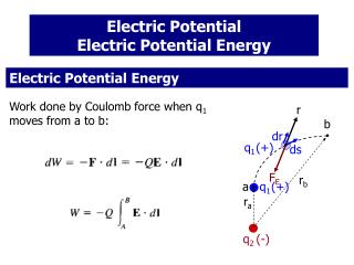
ELECTRIC POTENTIAL DIFFERENCE The fundamental definition of the electric potential V is given in terms of the electric field: B VAB = - ABE · dl A VAB = Electric potential difference between the points A and B = VB-VA. This is not the way we will usually calculate electric potentials, but we will explore this in a couple of simple examples to understand it better.
VAB = - AB E · dl Constant electric field E A dl • L • B The electric potential difference does not depend on the integration path. So pick a simple path. One possibility is to integrate along the straight line AB. This is easy in this case because E is constant and the anglebetween E and dl is constant. E · dl = E dl cos(p-) VAB = -E cos(p-) dl = E L cos
VAB = - AB E · dl VAB = E L cos Constant electric field E d A C • • q L • B This line integral is the same for any path connecting the same endpoints. For example, try the two-step path A to C to B. VAB = VAC + VCB VAC = E d VCB = 0 (E dl) Thus, VAB = E d but d = L cos Notice: the electric field points downhill
Equipotential Surfaces (lines) A E For a constant field E all of the points along the vertical line A are at the same potential.
Equipotential Surfaces (lines) A E For a constant field E all of the points along the vertical line A are at the same potential. Pf: DVbc=-∫E·dl=0 because Edl. We can say line A is at potential VA. b c
Equipotential Surfaces (lines) A x E For a constant field E all of the points along the vertical line A are at the same potential. Pf: DVbc=-∫E·dl=0 because Edl. We can say line A is at potential VA. The same is true for any vertical line: all points along it are at the same potential. For example, all points on the dotted line a distance x from A are at the same potential Vx, where VAx = E x
Equipotential Surfaces (lines) A x E For a constant field E all of the points along the vertical line A are at the same potential. Pf: DVbc=-∫E·dl=0 because Edl. We can say line A is at potential VA. The same is true for any vertical line: all points along it are at the same potential. For example, all points on the dotted line a distance x from A are at the same potential Vx, where VAx = E x A line (or surface in 3D) of constant potential is known as an Equipotential
Equipotential Surfaces We can make graphical representations of the electric potential in the same way as we have created for the electric field: Lines of constant E
Lines of constant V (perpendicular to E) Lines of constant E Equipotential Surfaces We can make graphical representations of the electric potential in the same way as we have created for the electric field:
Lines of constant V (perpendicular to E) Lines of constant E Equipotential Surfaces It is sometimes useful to draw pictures of equipotentials rather than electric field lines: Equipotential plots are like contour maps of hills and valleys. The electric field is the local slope, and points downhill.
Equipotential Surfaces How do the equipotential surfaces look for: (a) A point charge? E + (b) An electric dipole? - + Equipotential plots are like contour maps of hills and valleys. The electric field is the local slope, and points downhill.
Electric Potential of a Point Charge The Electric Potential b What is the electrical potential difference between two points (a and b) in the electric field produced by a point charge q? Point Charge q a q
Electric Potential of a Point Charge The Electric Potential b c Choose a path a-c-b. DVab = DVac + DVcb DVab = 0 because on this path Place the point charge q at the origin. The electric field points radially outwards. a q DVbc =
Electric Potential of a Point Charge The Electric Potential b c From this it’s natural to choose the zero of electric potential to be when ra Letting a be the point at infinity, and dropping the subscript b, we get the electric potential: a q When the source charge is q, and the electric potential is evaluated at the point r.
q Electric Potential of a Point Charge The Electric Potential Never do this derivation again. Instead, know this simple result by heart: r This is the most important thing to know about electric potential: the potential of a point charge q. Remember: this is the electric potential with respect to infinity – we chose V(∞) to be zero.
Potential Due to a Group of Charges • The second most important thing to know about electric potential is how to calculate it given more than one charge • For isolated point charges just add the potentials created by each charge (superposition) • For a continuous distribution of charge …
Potential Produced by aContinuous Distribution of Charge In the case of a continuous charge distribution, divide the distribution up into small pieces and then sum (integrate) the contribution from each bit: A r dVA = k dq / r VA = dVA = k dq / r dq Remember: k=1/(40)
P r z dw w R Example: a disk of charge dq = s2pwdw Suppose the disk has radius R and a charge per unit area s. Find the potential at a point P up the z axis (centered on the disk). Divide the object into small elements of charge and find the potential dV at P due to each bit. For a disk, a bit (differential of area) is a small ring of width dw and radius w.
Field and Electric Potential Remember from calculus that integrals are antiderivatives. By the fundamental theorem of calculus you can “undo” the integral: Given
Field and Electric Potential Remember from calculus that integrals are antiderivatives. By the fundamental theorem of calculus you can “undo” the integral: Given Very similarly you can get E(r) from derivatives of V(r).
Field and Electric Potential Remember from calculus that integrals are antiderivatives. By the fundamental theorem of calculus you can “undo” the integral: Given Very similarly you can get E(r) from derivatives of V(r). Choose V(r0)=0. Then
Field and Electric Potential Remember from calculus that integrals are antiderivatives. By the fundamental theorem of calculus you can “undo” the integral: Given Very similarly you can get E(r) from derivatives of V(r). Choose V(r0)=0. Then is the gradient operator The third most important thing to know about potentials.
Force and Potential Energy This is entirely analogous to the relationship between a conservative force and its potential energy. can be inverted: In a very similar way the electric potential and field are related by: can be inverted: The reason is that V is simply potential energy per unit charge.
P r z dw w R Example: a disk of charge • Suppose the disk has radius R and a charge per unit area s. • Find the potential and electric field at a point up the z axis. • Divide the object into small elements of charge and find the • potential dV at P due to each bit. So here let a bit be a small • ring of charge width dw and radius w. dq = s2pwdw
P r z dw w R Example: a disk of charge By symmetry one sees that Ex=Ey=0 at P. Find Ez from This is easier than integrating over the components of vectors. Here we integrate over a scalar and then take partial derivatives.
Example: point charge Put a point charge q at the origin. Find V(r): here this is easy: r q
Example: point charge Put a point charge q at the origin. Find V(r): here this is easy: r q Then find E(r) from the derivatives:
Example: point charge Put a point charge q at the origin. Find V(r): here this is easy: r q Then find E(r) from the derivatives: Derivative:
Example: point charge Put a point charge q at the origin. Find V(r): here this is easy: r q Then find E(r) from the derivatives: Derivative: So:
Energy of a Charge Distribution How much energy ( work) is required to assemble a charge distribution ?. CASE I: Two Charges Bringing the first charge does not require energy ( work)
Q2 Q1 r Energy of a Charge Distribution How much energy ( work) is required to assemble a charge distribution ?. CASE I: Two Charges Bringing the first charge does not require energy ( work) Bringing the second charge requires to perform work against the field of the first charge.
Q2 Q1 r Energy of a Charge Distribution CASE I: Two Charges Bringing the second charge requires to perform work against the field of the first charge. W = Q2 V1 with V1 = (1/40) (Q1/r) W = (1/40) (Q1 Q2/r) = U U = potential energy of two point charges U = (1/40) (Q1 Q2/r)
U12 = potential energy of a pair of point charges Energy of a Charge Distribution CASE II: Several Charges How much energy is stored in thissquare charge distribution?, or … What is the electrostatic potential energy of the distribution?, or … How much work is needed to assemble this charge distribution? Q Q Q Q a To answer it is necessary to add up the potential energy of each pair of charges U = Uij U12 = (1/40) (Q1 Q2/r)
-Q +Q Energy of a Charge Distribution fields cancel A CASE III: Parallel Plate Capacitor fields add E d fields cancel Electric Field E = / 0 = Q / 0 A ( = Q / A) Potential Difference V = E d = Q d / 0 A
-Q +Q Energy of a Charge Distribution fields cancel A CASE III: Parallel Plate Capacitor fields add E d fields cancel Now, suppose moving an additional very small positive charge dq from the negative to the positive plate. We need to do work. How much work? dW = V dq = (q d / 0 A) dq We can use this expression to calculate the total work neededto charge the plates to Q, -Q
-Q +Q Energy of a Charge Distribution fields cancel A CASE III: Parallel Plate Capacitor fields add E d fields cancel dW = V dq = (q d / 0 A) dq The total work neededto charge the plates to Q, -Q, is given by: W = dW = (q d / 0 A) dq = (d / 0 A) q dq W = (d / 0 A) [Q2 / 2] = d Q2 / 2 0 A
-Q +Q Where is the energy stored ? The energy is stored in the electric field W = U = d Q2 / 2 0 A Energy of a Charge Distribution fields cancel A CASE III: Parallel Plate Capacitor fields add E d fields cancel The work done in charging the plates ends up as stored potential energy of the final charge distribution
-Q +Q Energy of a Charge Distribution fields cancel A CASE III: Parallel Plate Capacitor fields add E d fields cancel The energy U is stored in the field, in the regionbetween the plates. E = Q / (0 A) U = d Q2 / 2 0 A = (1/2) 0 E2 A d The volume of this region is Vol = A d, so we can define the energy density uE as: uE = U / A d = (1/2) 0 E2
uE = U / A d = (1/2) 0 E2 Energy of a Charge Distribution Electric Energy Density CASE IV: Arbitrary Charge Distribution Although we derived this expression for the uniform field of a parallel plate capacitor, this is a universal expression valid for any electric field. When we have an arbitrary charge distribution, we can use uE to calculate the stored energy U . dU = uE d(Vol) = (1/2) 0 E2 d(Vol) U = (1/2) 0 E2 d(Vol) [The integral covers the entire region in which the field E exists]
A Shrinking Sphere A sphere of radius R1 carries a total charge Q distributed evenly over its surface. How much work does it take to shrink the sphere to a smaller radius R2 ?.