Download
1 / 8
80 likes | 162 Views
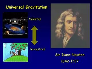
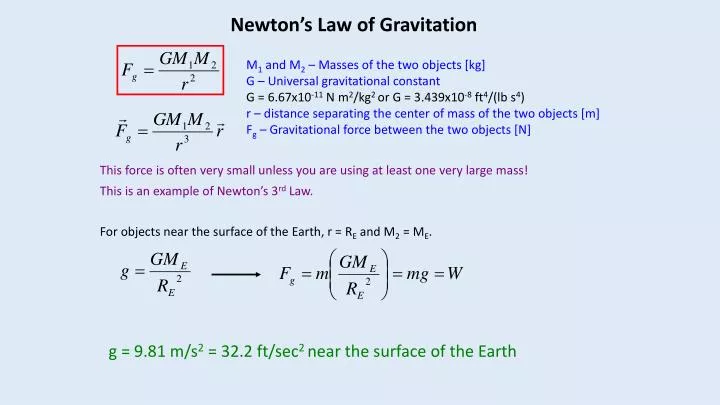
Newton’s Law of Gravitation. M 1 and M 2 – Masses of the two objects [kg] G – Universal gravitational constant G = 6.67x10 -11 N m 2 / kg 2 or G = 3.439x10 -8 ft 4 /( lb s 4 ) r – distance separating the center of mass of the two objects [m]

E N D
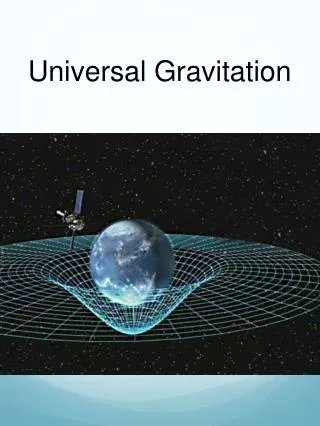
Newton’s Law of Gravitation M1 and M2 – Masses of the two objects [kg] G – Universal gravitational constant G = 6.67x10⁻¹¹ N m2/kg2or G = 3.439x10⁻⁸ft4/(lbs4) r – distance separating the center of mass of the two objects [m] Fg – Gravitational force between the two objects [N] This force is often very small unless you are using at least one very large mass! This is an example of Newton’s 3rd Law. For objects near the surface of the Earth, r = RE and M2 = ME. g = 9.81 m/s2 = 32.2 ft/sec2 near the surface of the Earth
Accuracy, Limits and Approximations Significant Figures: The precision of an answer cannot be more than the precision of the quantities used to determine the answer. Example: Measure the length of an object using a meterstick. What is the smallest length that can be measured (not estimated)? 1 mm – therefore all lengths measured with a meterstick are known to the nearest mm. Differentials: Differentials are used to describe infinitesimal pieces. Higher order differentials can often times be neglected. The use of higher order differentials is primarily to increase the precision of a measurement or when using multi-dimensional variables. Example: Let us examine a small quantity Dx, where Dx = 0.0001. Using the following expression y = ADx + BDx2 + CDx3, where A, B and C are constants, determine y. y = ADx + BDx2 + CDx3 = A(0.0001) + B(0.00000001) + C(0.000000000001) ≈ 0.0001A Also note that dx > dxdy > dxdydz Small Angle Approximation: For angles that are less than 20o it is acceptable to use a small angle approximation. - To use this approximation q must be expressed in radians! Sinq ≈ Tanq ≈ q Cosq≈ 1
Problem Solving • Use appropriate assumptions – Ex: Ignore weight of string if the Tension is much larger. • Use graphical analysis when appropriate (Charts, Diagrams, Graphical Solutions) • Aids in visualization • Means of presenting results • Remember to use appropriate scale • Draw a free-body diagram (proper techniques for this will be presented later) • Choose between numerical solution and symbolic solution • Symbolic solutions give a more general result and is more useful for discerning meaning • Numerical solutions are good for a one-time calculation, but the meaning is often obscured. • Problem Solving Steps: (order is not important) • Draw a Picture. • Choose your reference frame. • Identify known quantities. • Identify unknown quantities. • Identify equations that can be used to model this specific situation. • Solve the selected equation(s) for an unknown quantity. • Check numerical answer – for calculation errors. • Check units – use dimensional analysis. • Check significance of numerical value – Does it make sense? • Draw Conclusions
Chapter 2 Force Systems
In this section you will be expected to analyze a variety of situations using forces. Forces are vectors, so pay attention to magnitude, direction and point of application. We will only be concerned with forces applied externally to the defined system (internal forces sum to zero) and no deformation will occur on any object. Principle of Transmissibility: Applied forces can be slid along it’s line of action (line parallel to the direction of the force) without changing the outcome. Line of Action • Force Classification: Terms used to classify forces applied in a similar fashion. • Contact Forces – Forces applied directly to an object • Body Forces (field Forces) – Forces applied simultaneously to all points on an object (gravity, electric forces, magnetic forces, etc.) • Distributed Forces – Force applied over a specific geometric region (line, area or volume) of the object. • Concentrated Force – Distributed force over a geometric region that is much smaller than the size of the object and can therefore be considered applied at a single point.
Concurrent Forces: Lines of action of two or more forces intersect. Slide vectors along line of action until the tail of the vector is at the point of intersection and then sum vectorally. Forces F1 and F2 are concurrent since the vectors intersect at A. Forces F1 and F2 are concurrent since the lines of action intersect at A. Vector sum of F1 and F2 give a correct line of action for R. Vector sum of F1 and F2 give an incorrect line of action for R. Do not confuse vector components of R with projections of R onto an axis with the vector sum of two forces that are equivalent to R! F1 and F2 are vectors that when summed are equal to R. y Fx Fa and Fb are projections of R along the a and b axis, respectively. The axis a and b are not perpendicular! Fx and Fy are components of R along the x and y axis, respectively. The axis x and y are perpendicular! x Fy
When you have two parallel forces it is also necessary to determine the line of action for the resultant. The magnitude and direction can easily be determined from a vector sum of the two forces. The line of action/point of application of the resultant also needs to be determined. Add equal magnitude and oppositely directed forces to the two parallel forces. Determine a resultant R1 and R2 for each of the forces. Sum the two resultants R1 and R2 to determine the resulting force R. The point of intersection of the lines of action for the two resultants R1 and R2will indicate the point of application of R with the line of action parallel to R.
2D – Force Systems • Choose appropriate coordinate system for situation. Standard x-horizontal and y-vertical system may not be the best choice! • Relate forces to the chosen coordinate system using proper component notation. • Determine magnitude and direction of a vector from components.