Download
1 / 31
310 likes | 598 Views
Lecture 7: Z-transform. Instructor: Dr. Gleb V. Tcheslavski Contact: gleb@ee.lamar.edu Office Hours: Room 2030 Class web site: http://ee.lamar.edu/gleb/dsp/index.htm. Definitions.

E N D
Lecture 7: Z-transform Instructor: Dr. Gleb V. Tcheslavski Contact:gleb@ee.lamar.edu Office Hours: Room 2030 Class web site: http://ee.lamar.edu/gleb/dsp/index.htm
Definitions Z-transform converts a discrete-time signal into a complex frequency-domain representation. It is similar to the Laplace transform for continuous signals. (7.2.1) If (where) it exists! n is an integer time index; is a complex number; - angular freq. When the magnitude r =1, (7.2.2) If it exists!
Region of Convergence (ROC) The Region of convergence (ROC) is the set of points z in the complex plane, for which the summation is bounded (converges): (7.3.1) Since z is complex: (7.3.2) (7.3.3) In general, z-transform exists for (7.3.4) Im (7.3.5) r - r + Re
Region of Convergence (ROC) Examples of ROCs from Mitra
Region of Convergence (ROC) Example 7.1: Let xn = an There are no values of z satisfying: Example 7.2: Let xn = an un – a causal sequence (7.5.1) x ROC We can modify (7.5.1) as Im (7.5.2) a Re roots of numerator: X(z) = 0 roots of denominator: X(z)
Region of Convergence (ROC) Example 7.3: Let xn = -an u-n-1 – an anticausal sequence (7.6.1) Im x a Conclusion 1: z-transform exists only within the ROC! Re Conclusion 2: z-transform and ROC uniquely specify the signal. Conclusion 3: poles cannot exist in the ROC; only on its boundary. Note: if the ROC contains the unit circle (|z| = 1), the system is stable.
The transfer function Time shift: (7.7.1) Consider an LCCDE: (7.7.2) and take z-transform utilizing time shift (7.7.3) LTI: (7.7.4) The system transfer function (7.7.5)
Rational z-transform Frequently, a z-transform can be described as a rational function, i.e. a ratio of two polynomials in z-1: (7.8.1) Here M and N are the degrees of the numerator’s and denominator’s polynomials. An alternative representation is a ratio of two polynomials in z: (7.8.2) Finally, a rational z-transform can be written in a factorized form: zeros: numerator = 0 (7.8.3) Poles: denominator = 0
Notes on poles of a system function Positions of poles of a transfer function are used to evaluate system stability. Let assume a single real pole at z = . Therefore: (7.9.1) The difference equation is: (7.9.2) Therefore, the impulse response is: (7.9.3) for (7.9.4) Iff || < 1, hn decays as n and the system is BIBO stable; otherwise, hn grows without limits. Therefore, poles of a stable system (and signals in fact) must be inside the unit circle. Zeros may be placed anywhere. Zeros at the origin produce a time delay.
The transfer function and the Frequency response BIBO: (7.10.1) (7.10.2) where zjare zeros and pi are poles of the transfer function. BIBO: (7.10.3)
The transfer function and the Frequency response A good way to evaluate the system’s frequency response: (7.11.1) Zero-padded When the frequency approaches a pole, the frequency response has a local maximum, a zero forces the response to a local minimum. For real systems, poles and zeros are symmetrical with respect to the real axis. pole zero
The transfer function and the SFG (7.12.1) (7.12.2) (7.12.3) Poles of H(z) correspond to the eigenvalues of the system matrix.
More on Transfer function zeros (7.13.1) poles • N > M: zeros at z = 0 of multiplicity N-M • M > N: poles at z = 0 of multiplicity M-N (7.13.2)
Types of digital filters 1. FIR (“all-zero”) filter: (7.14.1) All poles are at z = 0: a “nest of poles” ROC: the entire z-plane except of the origin (z = 0). FIR filters are stable.
Types of digital filters 2. IIR (“all-pole”) filter: (7.15.1) All zeros are at z = 0: a “nest of zeros”
Types of digital filters 3. General IIR (“zero-pole”) filter: (7.16.1)
On test signals… (7.17.1) (7.17.2) (7.17.3) Calculate and compare to We don’t need any other that a delta function test signals since a unit-pulse response is a complete system’s description.
Types of sequences and convergence 1. Two-sided: (7.18.1) Converges everywhere except of z = 0 and z =
Types of sequences and convergence 2. Right-sided: Blows up at z = (7.19.1) Assume: if converges at z = z0, converges for |z| > | z0| ROC: r - < |z| < - exterior ROC For a causal sequence: |z| > r - = max|pk| - a max pole of G(z) To be causal, a sequence must be right-sided (necessary but not sufficient)
Types of sequences and convergence 3. Left-sided: (7.20.1) Converges at z0 Blows up at z = 0 ROC: 0 < |z| < r + - interior ROC When encountering an interior ROC, we need to check convergence at z = 0. If the sequence “blows up” at zero – it’s an anti-causal sequence
Properties from Mitra
Inverse z-transform (7.23.1) Where C is a counterclockwise closed path encircling the origin and is entirely in the ROC. Contour C must encircle all the poles of X(z). In general, there is no simple way to compute (7.23.1) A special case: C is the unit circle (can be used when the ROC includes the unit circle). The inverse z-transform reduces to the IDTFT. (7.23.2)
Inverse z-transform A. Via Cauchy residue theorem (7.24.1) For all poles of X(z)zn-1 inside C (contour of integration) Where i are the residues of X(z)zn-1 for a pole of multiplicity k: (7.24.2) Residue function: (7.24.3)
Inverse z-transform: Example Example: Im C x 0 is a residue of X(z)z-n-1 at z=0 – involves pole of multiplicity –n wnen n < 0. a Re multiplicity
Inverse z-transform B. Via recognition (table look-up) Sometimes, the z-transform can be modified such way that it can be found in a table… Example: Therefore:
Inverse z-transform C. Via long division 1. Right-sided z-transform sequences can be expanded into a power series in z-1. The coefficient multiplying z-n is the nth sample of the inverse z-transform. Example: Lower powers first: and long division: x0 x1 x2 x3 x4
Inverse z-transform 2. Left-sided z-transform sequences – into a power series in z1… Example: Multiply both numerator and denominator by z2 … Long division… x0 x-1 x-2 x-3 x-4 x1 Non-causal
Inverse z-transform Example: not suitable for long division! Example:
Inverse z-transform D. Via partial fraction expansion (PFE) (7.30.1) If the degree of the numerator is equal or greater than the degree of the denominator: M N, G(z) is an improper polynomial. Then: (7.30.2) A proper fraction: M1 < N Then: (7.30.3) Simple poles: multiplicity of 1.
Inverse z-transform Here l is a residue (7.31.1) poles Therefore: (7.31.2) This method is suitable for complex poles. Problem: large polynomials are hard to manipulate… ??QUESTIONS??