Download
1 / 40
410 likes | 885 Views
Biological networks: Types and sources. Protein-protein interactions, Protein complexes, and network properties. Networks in electronics. Lazebnik, Cancer Cell, 2002. Model Generation. Interactions. Sequencing Gene knock-out Microarrays etc. YER001W YBR088C YOL007C YPL127C

E N D
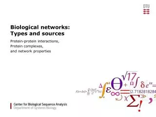
Biological networks:Types and sources Protein-protein interactions, Protein complexes, and network properties
Networks in electronics Lazebnik, Cancer Cell, 2002
Model Generation Interactions • Sequencing • Gene knock-out • Microarrays • etc. YER001W YBR088C YOL007C YPL127C YNR009W YDR224C YDL003W YBL003C … YDR097C YBR089W YBR054W YMR215W YBR071W YBL002W YNL283C YGR152C … Parts List • Genetic interactions • Protein-Protein interactions • Protein-DNA interactions • Subcellular Localization Interactions • Microarrays • Proteomics • Metabolomics Dynamics Lazebnik, Cancer Cell, 2002
Protein-protein interactions Protein-DNA interactions Genetic interactions Metabolic reactions Co-expression interactions Text mining interactions Association networks Interaction networks in molecular biology
Approaches by interaction/method type • Physical Interactions • Yeast two hybrid screens (PPI) • Affinity purification mass spectrometry, APMS (PPI) • Protein complementation assays (PPI) • ChIP-Seq, ChIP-Chip (protein-DNA) • CLIP-Seq, RIP-Seq, HITS-CLIP, PAR-CLIP (protein-RNA) • Other measures of ‘association’ • Genetic interactions (double deletion mutants) • Co-expression • Functional associations • STRING (which includes many of the above and more)
Yeast two-hybrid method Y2H assays interactions in vivo. Uses property that transcription factors generally have separable transcriptional activation (AD) and DNA binding (DBD) domains. A functional transcription factor can be created if a separately expressed AD can be made to interact with a DBD. A protein ‘bait’ B is fused to a DBD and screened against a library of protein “preys”, each fused to a AD.
Issues with Y2H • Strengths • Takes place in vivo • Independent of endogenous expression • Weaknesses: False positive interactions • Detects “possible interactions” that may not take place under physiological conditions • May identify indirect interactions (A-C-B) • Weaknesses: False negatives interactions • Similar studies often reveal very different sets of interacting proteins (i.e. False negatives) • May miss PPIs that require other factors to be present (e.g. ligands, proteins, PTMs)
Protein interactions by immunoprecipitation followed by mass spectrometry (APMS) • Start with affinity purification of a single epitope-tagged protein • This enriched sample typically has a low enough complexity to be fractionated by electrophoresis techniques
Affinity Purification Mass Spec • Strengths • High specificity • Well suited for detecting permanent or strong transient interactions (complexes) • Detects real, physiologically relevant PPIs • Weaknesses • Lower sensitivity: Less suited for detecting weaker transient interactions • May miss complexes not present under the given experimental conditions (low sensitivity) • May identify indirect interactions (A-C-B)
Recent binary PPI network Y2H by Yu et al. 2008 : 2018 proteins, 2930 interactions PCA by Tarassov et al. 2008 : 1124 proteins, 2770 interactions
Other characterizations of physical interactions • Obligation • obligate (only found/function together) • non-obligate (can exist/function alone) • Time of interaction • permanent (complexes, often obligate) • strong transient (require trigger, e.g. G proteins) • weak transient (dynamic equilibrium) • Location/compartmentalization constraints • Same/different cellular compartment • Tissue specificity
iRefIndex integration of PPI DBshttp://irefindex.uio.no/wiki/iRefIndex
Filtering by subcellular localization de Lichtenberg et al., Science, 2005
D A B C High confidence (1 unshared interaction partners) Low confidence (4 unshared interaction partners) An example binary-interaction score • For the yeast two-hybrid experiments, the reliability of an interaction has been found to correlate well with the number of non-shared interaction partners for each interactor [6]. This can be summarized in the following raw quality score • where NA and NB are the numbers of non-shared interaction partners for an interaction between protein A and B.
An example “pull-down” interaction score • For APMS or other IP pull-down experiments, the reliability of the inferred binary interactions has been found to correlate better with the number of times the proteins were co-purified vs. purified individually. • where: • NAB is the number of purifications containing both proteins, i.e. the intersection of experiments that find them, • NAB is the total number of purifications that find either A or B, i.e. the union of experiments that find them, • NA is the number of purifications containing A, and • NB is the numbers of purifications containing B
Network Properties Graphs, paths, topology
Graphs • Graph G=(V,E) is a set of vertices V and edges E • A subgraph G’ of G is induced by some V’V and E’ E • Graph properties: • Connectivity (node degree, paths) • Cyclic vs. acyclic • Directed vs. undirected
Sparse vs Dense • G(V, E) • Where |V|=n the number of vertices • And |E|=m the number of edges • Graph is sparse if m ~ n • Graph is dense if m ~ n2 • Complete graph when m = (n2-n)/2 ~ n2
Connected Components • G(V,E) • |V| = 69 • |E| = 71
Connected Components • G(V,E) • |V| = 69 • |E| = 71 • 6 connected components
Paths A path is a sequence {x1, x2,…, xn} such that (x1,x2), (x2,x3), …, (xn-1,xn) are edges of the graph. A closed path xn=x1 on a graph is called a graph cycle or circuit.
Degree or connectivity Barabási AL, Oltvai ZN. Network biology: understanding the cell's functional organization. Nat Rev Genet. 2004 Feb;5(2):101-13
Random vs scale-free networks P(k) is probability of each degree k, i.e fraction of nodes having that degree. For random networks, P(k) is normally distributed. For real networks the distribution is often a power-law: P(k) ~ k-g Such networks are said to be scale-free Barabási AL, Oltvai ZN. Network biology: understanding the cell's functional organization. Nat Rev Genet. 2004 Feb;5(2):101-13
Clustering coefficient The density of the network surrounding node I, characterized as the number of triangles through I. Related to network modularity k: neighbors of I nI: edges between node I’s neighbors The center node has 8 neighbors (green) There are 4 edges between these neighbors C = 1/7
Proteins subunits are highly interconnected and thus have a high clustering coefficient There exists algorithms, such as MCODE, for identifying subnetworks (complexes) in large protein-protein interaction networks Protein complexes have a high clustering coefficient
Hierarchical Networks Barabási AL, Oltvai ZN. Nat Rev Genet. 2004
Detecting hierarchical organization Barabási AL, Oltvai ZN. Nat Rev Genet. 2004
Scale-free networks are robust • Complex systems (cell, internet, social networks), are resilient to component failure • Network topology plays an important role in this robustness • Even if ~80% of nodes fail, the remaining ~20% still maintain network connectivity • Attack vulnerability if hubs are selectively targeted
Other interesting features • Cellular networks are assortative, i.e. hubs tend not to interact directly with other hubs. • Hubs have been claimed to be “older” proteins (so far claimed for protein-protein interaction networks only) • Hubs also seem to have more evolutionary pressure—their protein sequences are more conserved than average between species (shown in yeast vs. worm)