Download
1 / 29
290 likes | 432 Views
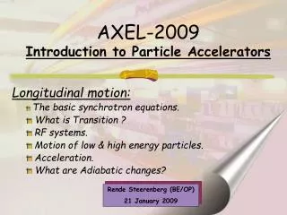
AXEL- 2013 Introduction to Particle Accelerators. Resonances: Normalised Phase Space Dipoles, Quadrupoles, Sextupoles A more rigorous approach Coupling Tune diagram. Rende Steerenberg (BE/OP) 24 April 2013. b y ’. Circle of radius. y. Normalised Phase Space.

E N D
AXEL-2013Introduction to Particle Accelerators Resonances: Normalised Phase Space Dipoles, Quadrupoles, Sextupoles A more rigorous approach Coupling Tune diagram Rende Steerenberg (BE/OP) 24 April 2013
by’ Circle of radius y Normalised Phase Space • By multiplying the y-axis by β the transverse phase space is normalised and the ellipse turns into a circle. AXEL - 2013
y by’ 2p 0 y Phase Space & Betatron Tune • If we unfold a trajectory of a particle that makes one turn in our machine with a tune of Q = 3.333, we get: • This is the same as going 3.333 time around on the circle in phase space • The net result is 0.333 times around the circular trajectory in the normalised phase space • q is the fractional part of Q • So here Q= 3.333 and q = 0.333 2πq AXEL - 2013
What is a resonance? • After a certain number of turns around the machine the phase advance of the betatron oscillation is such that the oscillation repeats itself. • For example: • If the phase advance per turn is 120º then the betatron oscillation will repeat itself after 3 turns. • This could correspond to Q = 3.333 or 3Q = 10 • But also Q = 2.333 or 3Q = 7 • The order of a resonance is defined as ‘n’ n x Q = integer AXEL - 2013
Q = 3.333 in more detail 1st turn 2nd turn 3rd turn Third order resonant betatron oscillation 3Q = 10, Q = 3.333, q = 0.333 AXEL - 2013
Q = 3.333 in Phase Space • Third order resonance on a normalised phase space plot 2nd turn 3rd turn 1st turn 2πq = 2π/3 AXEL - 2013
Machine imperfections • It is not possible to construct a perfect machine. • Magnets can have imperfections • The alignment in the de machine has non zero tolerance. • Etc… • So, we have to ask ourselves: • What will happen to the betatron oscillation s due to the different field errors. • Therefore we need to consider errors in dipoles, quadrupoles, sextupoles, etc… • We will have a look at the beam behaviour as a function of ‘Q’ • How is it influenced by these resonant conditions? AXEL - 2013
y’b Q = 2.00 Q = 2.50 y y Dipole (deflection independent of position) y’b 1st turn 2nd turn 3rd turn • For Q = 2.00: Oscillation induced by the dipole kick grows on each turn and the particle is lost (1st order resonance Q = 2). • For Q = 2.50: Oscillation is cancelled out every second turn, and therefore the particle motion is stable. AXEL - 2013
Q = 2.50 Q = 2.33 1st turn 2nd turn 3rd turn 4th turn Quadrupole (deflection position) • For Q = 2.50: Oscillation induced by the quadrupole kick grows on each turn and the particle is lost (2nd order resonance 2Q = 5) • For Q = 2.33: Oscillation is cancelled out every third turn, and therefore the particle motion is stable. AXEL - 2013
Q = 2.25 Q = 2.33 1st turn 2nd turn 3rd turn 4th turn 5th turn Sextupole (deflection position2) • For Q = 2.33: Oscillation induced by the sextupole kick grows on each turn and the particle is lost (3rd order resonance 3Q = 7) • For Q = 2.25: Oscillation is cancelled out every fourth turn, and therefore the particle motion is stable. AXEL - 2013
y’b θ a y Dby’ 2πDQ Da More rigorous approach (1) • Let us try to find a mathematical expression for the amplitude growth in the case of a quadrupole error: 2πQ = phase angle over 1 turn = θ Δβy’ = kick a = old amplitude Δa = change in amplitude 2πΔQ = change in phase y does not change at the kick y = a cos(θ) θ In a quadrupole Δy’ = lky Only if 2πΔQ is small So we have: Δa = βΔy’ sin(θ) = lβ sin(θ) a k cos(θ) AXEL - 2013
a = l··sin() a·k·cos() • So we have: and thus: More rigorous approach (2) • Each turn θ advances by 2πQ • On the nth turn θ = θ + 2nπQ Sin(θ)Cos(θ) = 1/2 Sin (2θ) • Over many turns: This term will be ‘zero’ as it decomposes in Sin and Cos terms and will give a series of + and – that cancel out in all cases where the fractional tune q ≠ 0.5 • So, for q = 0.5 the phase term, 2(θ + 2nπQ) is constant: AXEL - 2013
More rigorous approach (3) • In this case the amplitude will grow continuously until the particles are lost. • Therefore we conclude as before that: quadrupolesexcite 2nd order resonances for q=0.5 • Thus for Q = 0.5, 1.5, 2.5, 3.5,…etc…… AXEL - 2013
y’b θ a y Dby’ Da 2πDQ More rigorous approach (4) • Let us now look at the phase θfor the same quadrupole error: 2πQ = phase angle over 1 turn = θ Δβy’ = kick a = old amplitude Δa = change in amplitude 2πΔQ= change in phase y does not change at the kick y = a cos(θ) θ In a quadrupole Δy’ = lky s 2πΔQ << Therefore Sin(2πΔQ) ≈ 2πΔQ AXEL - 2013
So we have: • Since: we can rewrite this as: , which is correct for the 1st turn • Over many turns: ‘zero’ • Averaging over many turns: More rigorous approach (5) • Each turn θ advances by 2πQ • On the nth turn θ = θ + 2nπQ AXEL - 2013
, which is the expression for the change in Q due to a quadrupole… (fortunately !!!) • But note that Q changes slightly on each turn Related to Q Max variation 0 to 2 • Q has a range of values varying by: Stopband • This width is called the stopbandof the resonance • So even if q is not exactly 0.5, it must not be too close, or at some point it will find itself at exactly 0.5 and ‘lock on’ to the resonant condition. AXEL - 2013
and thus • For a sextupole • We get : • Summing over many turns gives: 1st order resonance term 3rd order resonance term • Sextupole excite 1st and 3rdorder resonance q = 0.33 q = 0 Sextupole kick • We can apply the same arguments for a sextupole: AXEL - 2013
and thus • For an octupole 4th order resonance term • We get : 2nd order resonance term • Summing over many turns gives: a2(cos 4(+2pnQ) + cos 2(+2pnQ)) Amplitude squared q = 0.5 q = 0.25 • Octupolar errors excite 2nd and 4thorder resonance and are very important for larger amplitude particles. Octupole kick • We can apply the same arguments for an octupole: Can restrict dynamic aperture AXEL - 2013
Resonance summary • Quadrupoles excite 2nd order resonances • Sextupoles excite 1st and 3rd order resonances • Octupoles excite 2nd and 4th order resonances • This is true for small amplitude particles and low strength excitations • However, for stronger excitations sextupoles will excite higher order resonance’s (non-linear) AXEL - 2013
Coupling • Coupling is a phenomena, which converts betatron motion from one plane (horizontal or vertical) into motion in the other plane. • Fields that will excite coupling are: • Skew quadrupoles, which are normal quadrupoles, but tilted by 45º about it’s longitudinal axis. • Solenoidal (longitudinal magnetic field) AXEL - 2013
S N N S Skew Quadrupole Magnetic field Like a normal quadrupole, but then tilted by 45º AXEL - 2013
Solenoid; longitudinal field (2) Particle trajectory Magnetic field Beam axis Transverse velocity component AXEL - 2013
Solenoid; longitudinal field (2) Above: The LPI solenoid that was used for the initial focusing of the positrons. It was pulsed with a current of 6 kA for some 7 υs, it produced a longitudinal magnetic field of 1.5 T. At the right: The somewhat bigger CMS solenoid AXEL - 2013
Coupling and Resonance • This coupling means that one can transfer oscillation energy from one transverse plane to the other. • Exactly as for linear resonances there are resonant conditions. • If we meet one of these conditions the transverse oscillation amplitude will again grow in an uncontrolled way. nQh mQv = integer AXEL - 2013
General tune diagram 2Qv =5 Qv Qh - Qv= 0 2.75 2.5 4Qh =11 2.25 2 2 2.25 2.5 2.75 Qh 2.66 2.33 AXEL - 2013
Realistic tune diagram injection During acceleration we change the horizontal and vertical tune to a place where the beam is the least influenced by resonances. ejection AXEL - 2013
Measured tune diagram Move a large emittance beam around in this tune diagram and measure the beam losses. Not all resonance lines are harmful. AXEL - 2013
Conclusion • There are many things in our machine, which will excite resonances: • The magnets themselves • Unwanted higher order field components in our magnets • Tilted magnets • Experimental solenoids (LHC experiments) • The trick is to reduce and compensate these effects as much as possible and then find some point in the tune diagram where the beam is stable. AXEL - 2013
Questions….,Remarks…? Resonance Phase space Coupling Tune diagram AXEL - 2013