Download
1 / 19
190 likes | 354 Views
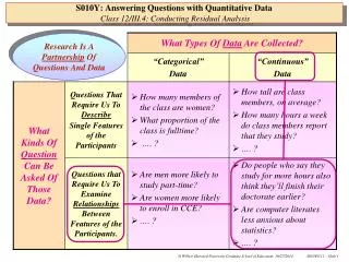
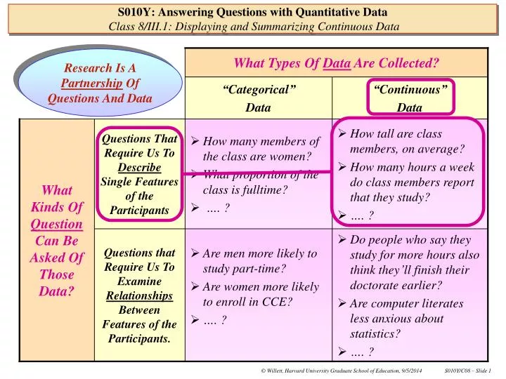
What Types Of Data Are Collected?. Research Is A Partnership Of Questions And Data. “Categorical” Data. “Continuous” Data. S010Y: Answering Questions with Quantitative Data Class 8/III.1: Displaying and Summarizing Continuous Data. What Kinds Of Question Can Be Asked Of Those Data?.

E N D
What Types Of Data Are Collected? Research Is A Partnership Of Questions And Data “Categorical” Data “Continuous” Data S010Y: Answering Questions with Quantitative DataClass 8/III.1: Displaying and Summarizing Continuous Data What Kinds Of Question Can Be Asked Of Those Data? Questions That Require Us To Describe Single Features of the Participants • How many members of the class are women? • What proportion of the class is fulltime? • …. ? • How tall are class members, on average? • How many hours a week do class members report that they study? • …. ? Questions that Require Us To Examine Relationships Between Features of the Participants. • Are men more likely to study part-time? • Are women more likely to enroll in CCE? • …. ? • Do people who say they study for more hours also think they’ll finish their doctorate earlier? • Are computer literates less anxious about statistics? • …. ?
It is more difficult to summarize the sample distribution of a continuous variable, like MAT score, than it is to summarize the sample distribution of a categorical variable, because the sample distributions of continuous variables like MAT scores have so many interesting properties, including: • The “one-sidedness” of the batch. • The “peakiness” of the batch. • The “center” or “location” of the batch. • The “spread” of the batch. We have distinguished two broad approaches for creating statistical summaries of these properties: • Approach #2 • Based on thearithmetic manipulation of data values: • Mean, standard deviation, skewness, kurtosis, … • Approach #1 • Based on theordering of data values: • Median, quartiles, percentiles, inter-quartile range, … • Last time, I focused on generating such summaries using the ordering principle. • Today, I’ll focus on generating summaries using the arithmetic manipulation principle. S010Y: Answering Questions with Quantitative DataClass 8/III.1: Displaying and Summarizing Continuous Data
9 8 7 6 5 4 3 2 1 2 3 3 9 6 0 7 8 8 9 8 1 0 0 0 1 6 6 8 0 3 6 0 5 0 7 5 3 7 2 0 0 7 9 1 0 9 8 7 6 5 4 3 2 1 9 1 A good summary statistic for describing the center of a distribution of the values of a continuous variable is theplace where the distribution would need to be supported so that it could “balance.” Let’s use the arithmetic principle to develop a statistic for describing the center of the distributionof the values of a continuous variable like MAT score … for the “Early” “Elsewhere” batch, for instance … S010Y: Answering Questions with Quantitative DataClass 8/III.1: Displaying and Summarizing Continuous Data
9 6 8 1 6 8 0 3 0 7 5 3 2 0 0 7 9 1 0 9 8 7 6 5 4 3 2 1 A good summary statistic for describing the center of the distribution of the values of a continuous variable, like MAT score, is the place where the distribution must be supported for it to balance S010Y: Answering Questions with Quantitative DataClass 8/III.1: Displaying and Summarizing Continuous Data Known as the sample mean, or average.
Why don’t we just find the average distance of all the “blocks”from thecenter? 9 6 8 1 6 8 0 3 0 7 5 3 2 0 0 7 9 1 0 9 8 7 6 5 4 3 2 1 let’s use the arithmetic principle to create a summary statistic for describing the spread of the distribution of values of a continuous variable … how about the “average distance from the center”? S010Y: Answering Questions with Quantitative DataClass 8/III.1: Displaying and Summarizing Continuous Data
9 6 8 1 6 8 0 3 0 7 5 3 2 0 0 7 9 1 0 9 8 7 6 5 4 3 2 1 Now I guess we should take the square root, to reverse the squaring that we did to begin with? Let’s call this the standard deviation. When you sum, everything goes to zero, so what do we do now …. ? Let’s do what we’ve done before, square all the distances before averaging? S010Y: Answering Questions with Quantitative DataClass 8/III.1: Displaying and Summarizing Continuous Data
9 6 8 1 1 standard deviation 6 8 0 3 0 7 5 3 2 0 0 7 9 1 0 9 8 7 6 5 4 3 2 1 Mean 63.4 80.1 46.7 And so, creating summary statistics based on the arithmetic principle, here’s the story so far…... S010Y: Answering Questions with Quantitative DataClass 8/III.1: Displaying and Summarizing Continuous Data
When the test was received in the Admissions Office: • 1 = Early • 2 = Late Raw MAT score Entering cohort: 1 =1987 2 =1989 Location of test site: 1 = Harvard 2 = Elsewhere ID label • You don’t have to do all these computations by hand – SAS can do them for you: • Here are the MAT data you worked with, supplemented by data from the 1987 cohort. • All in the MAT.txtdataset. 1 01 1 64 2 1 02 1 54 2 1 03 1 93 2 1 04 1 82 2 1 05 1 75 2 1 06 1 72 2 1 07 1 59 2 1 08 1 76 2 1 09 1 38 2 1 10 1 73 2 1 11 1 88 2 1 12 1 50 1 1 13 1 96 1 1 14 1 66 1 1 15 1 93 1 1 16 1 63 1 (74 cases omitted) S010Y: Answering Questions with Quantitative DataClass 8/III.1: Displaying and Summarizing Continuous Data
Standard data input statements, notice that there are several other variables in the dataset The usual process of formatting the categorical variables Here’s a PC-SAS program to provide descriptive univariate statistics on these data … Handout C08_1 OPTIONS Nodate Pageno=1; TITLE1 ‘S010Y: Answering Questions with Quantitative Data'; TITLE2 'Class 8/Handout 1: Displaying and Summarizing Continuous Data, Part I'; TITLE3 'MAT Scores from 2 Years of Doctoral Applicants'; TITLE4 'Data in MAT.txt'; *-----------------------------------------------------------------------------* Input data, name and label variables in dataset *-----------------------------------------------------------------------------*; DATA MAT; INFILE 'C:\DATA\S010Y\MAT.txt'; INPUT YEARTEST ID WHENRECD MATSCOR TESTSITE; LABEL ID = 'Case identification number' YEARTEST = 'Year test taken' WHENRECD = 'When application received' MATSCOR = 'Millers Analogies Test Score' TESTSITE = 'Test site'; *-----------------------------------------------------------------------------* Format labels for values of categorical variables *-----------------------------------------------------------------------------*; PROC FORMAT; VALUE YEARFMT 1='1987' 2='1989'; VALUE WHENFMT 1='Early' 2='Late'; VALUE SITEFMT 1='Harvard' 2='Elsewhere'; S010Y: Answering Questions with Quantitative DataClass 8/III.1: Displaying and Summarizing Continuous Data
PROC UNIVARIATE provides all kind of univariate (“single variable”) descriptive statistics for continuous variables Printing, titling and formatting a few cases for inspection The PLOT command requests various data plots, including the stem.leaf plot. The VAR command specifies the continuous variable to be summarized The ID command identifies a variables that contains respondent identifying information And here’s the rest of the PC_SAS program … this part provides the requested univariate descriptive statistics ... *--------------------------------------------------------------------------* Data Listing *--------------------------------------------------------------------------*; PROC PRINT LABEL DATA=MAT; TITLE5 'Listing of MAT Scores & Background Variables for all Applicants'; VAR ID YEARTEST WHENRECD TESTSITE MATSCOR; FORMAT YEARTEST YEARFMT. WHENRECD WHENFMT. TESTSITE SITEFMT.; *--------------------------------------------------------------------------* Displaying and summarizing the MAT scores for the whole sample *--------------------------------------------------------------------------*; PROC UNIVARIATE PLOT DATA=MAT; TITLE5 'Univariate Descriptive Summaries of MAT Score for all Applicants'; VAR MATSCOR; ID ID; RUN; S010Y: Answering Questions with Quantitative DataClass 8/III.1: Displaying and Summarizing Continuous Data
Harvard graduation, 1890 The six class day speakers; with W.E.B. Du Bois on the far right Each row is a case, as usual Here’s a listing of a few cases from the dataset … S010Y: Answering Questions with Quantitative Data Class 8/Handout 1: Displaying and Summarizing Continuous Data, Part I MAT Scores from 2 Years of Doctoral Applicants Data in MAT.txt Listing of MAT Scores and Background Variables for all Applicants Case Year When Millers identification test application Analogies Obs number taken received Test site Test Score 1 1 1987 Early Elsewhere 64 2 2 1987 Early Elsewhere 54 3 3 1987 Early Elsewhere 93 4 4 1987 Early Elsewhere 82 5 5 1987 Early Elsewhere 75 6 6 1987 Early Elsewhere 72 7 7 1987 Early Elsewhere 59 8 8 1987 Early Elsewhere 76 9 9 1987 Early Elsewhere 38 10 10 1987 Early Elsewhere 73 . . 83 83 1989 Late Elsewhere 55 84 84 1989 Late Harvard 72 85 85 1989 Late Elsewhere 32 86 86 1989 Late Elsewhere 53 87 87 1989 Late Elsewhere 76 88 88 1989 Late Elsewhere 62 89 89 1989 Late Elsewhere 78 90 90 1989 Late Elsewhere 54 S010Y: Answering Questions with Quantitative DataClass 8/III.1: Displaying and Summarizing Continuous Data
The sample mean of MATSCOR is 63.39 The median (or 50th percentile) of MATSCOR is 65 The sample standard deviation of MATSCOR is 18.69. • The inter-quartilerange is the difference between the upper and lower quartiles: • Lower quartile = 53 • Upper quartile = 77 • Inter-quartile range = (77-53) = 24 • The range is the difference between the minimum and the maximum: • Minimum = 18 • Maximum = 96 • Range = (96-18) = 78 And the “ordering” and “arithmetic manipulation” summary statistics for MATSCOR are … Variable: MATSCOR (Millers Analogies Test Score) Moments N 90 Sum Weights 90 Mean 63.3888889 Sum Observations 5705 Std Deviation 18.6924815 Variance 349.408864 Skewness -0.5406701 Kurtosis -0.320241 Basic Statistical Measures Location Variability Mean 63.38889 Std Deviation 18.69248 Median 65.00000 Variance 349.40886 Mode 62.00000 Range 78.00000 Interquartile Range 24.00000 Quantiles Quantile Estimate 100% Max 96.0 99% 96.0 95% 90.0 90% 85.5 75% Q3 77.0 50% Median 65.0 25% Q1 53.0 10% 35.0 5% 27.0 1% 18.0 0% Min 18.0 S010Y: Answering Questions with Quantitative DataClass 8/III.1: Displaying and Summarizing Continuous Data
This is scientific notation: And don’t forget the inverses … 1.8 x 101 = 18, etc. Here’s SAS’s version of the stem.leaf plot for the values of MATSCOR … Millers Analogies Test Score Stem Leaf # 9 6 1 9 00333 5 8 5689 4 8 222334 6 7 556667788899 12 7 0011122223344 13 6 55669 5 6 000122223444 12 5 556899 6 5 00333444 8 4 57 2 4 022 3 3 55889 5 3 124 3 2 7 1 2 114 3 1 8 1 ----+----+----+----+ Multiply Stem.Leaf by 10**+1 S010Y: Answering Questions with Quantitative DataClass 8/III.1: Displaying and Summarizing Continuous Data
100 90 80 70 60 50 40 30 20 10 • Recall that, for the full sample (n=90) …. • Minimum, Maximum, & Range: • Min = 18 • Max = 96 • Range =78 • Quartiles, Median & Inter-Quartile Range: • 25 %ile Q1 = 53 • Median = 65 • 75 %ile Q3 = 77 • Interquartile Range = 24 • Mean: • Mean = 63.4 We can bring several of these univariate descriptive statistics – both the “ordering” and “arithmetic manipulation” versions -- together in a useful single summary figure called the “box and whisker” plot, or boxplot… S010Y: Answering Questions with Quantitative DataClass 8/III.1: Displaying and Summarizing Continuous Data
And here’s the PROC UNIVARIATE version of the box-plot from the previous handout….. The UNIVARIATE Procedure Variable: MATSCOR (Millers Analogies Test Score) Stem Leaf # Boxplot 9 6 1 | 9 00333 5 | 8 5689 4 | 8 222334 6 | 7 556667788899 12 +-----+ 7 0011122223344 13 | | 6 55669 5 *-----* 6 000122223444 12 | + | 5 556899 6 | | 5 00333444 8 +-----+ 4 57 2 | 4 022 3 | 3 55889 5 | 3 124 3 | 2 7 1 | 2 114 3 | 1 8 1 | ----+----+----+----+ Multiply Stem.Leaf by 10**+1 S010Y: Answering Questions with Quantitative DataClass 8/III.1: Displaying and Summarizing Continuous Data • What would the box-plot look like if the sample distribution of MATSCOR were perfectly symmetrical? • What would the box-plot look like if there was very little variability in MATSCOR in the sample? • What features of the sample distribution of MATSCOR account for the fact that the sample mean is smaller than the sample median?
Mean -2sd Mean - 1sd Mean Mean +1sd Mean +2sd An interesting aside on the normal distribution ….. Normal distribution simulation • A considerable number of continuous variables that occur “naturally” turn out to be “normally distributed”: • Height • Weight, • Test Scores, • Opinions, etc.… There is a special relationship between percentiles and standard deviation in a normal distribution S010Y: Answering Questions with Quantitative DataClass 8/III.1: Displaying and Summarizing Continuous Data If you were to plot a vertical histogram of the values of variables like these, you would get the familiar “bell-shaped curve”… Ball-drop simulation
Here, I’ve picked out only applicants in the 1989 (YEARTEST = 2) cohort, so that the new analyses will match the analyses that you conducted in original Activity #1. Let’s use categorical variables WHENRECD and TESTSITE to sub-divide the sample, so that we cancompare sub-sample distributions of MATSCOR using boxplots … like original Activity #1. The boxplot is very useful if you want to compare sample distributions of a continuous variable like MATSCOR across different groups, as in Activity #1 – see Handout C08_2 … OPTIONS Nodate Pageno=1; TITLE1 'S010Y: Answering Questions with Quantitative Data'; TITLE2 'Class 8/Handout 2: Displaying and Summarizing Continuous Data, Part II'; TITLE3 'Using Boxplots To Compare MAT Scores of Doctoral Applicants to APSP'; TITLE4 'Data in MAT.txt'; *-----------------------------------------------------------------------------* Input data, name and label variables in dataset *-----------------------------------------------------------------------------*; DATA MAT; INFILE 'C:\DATA\S010Y\MAT.txt'; INPUT YEARTEST ID WHENRECD MATSCOR TESTSITE; IF YEARTEST = 2; * Pick out 1989 Cohort for comparison with Activity #1; LABEL ID = 'Case identification number' YEARTEST = 'Year test taken' WHENRECD = 'When application received' MATSCOR = 'Millers Analogies Test Score' TESTSITE = 'Test site'; *-----------------------------------------------------------------------------* Format labels for the values of the categorical variables *-----------------------------------------------------------------------------*; PROCFORMAT; VALUE WHENFMT 1='Early' 2='Late'; VALUE SITEFMT 1='Harvard' 2='Elsewhere'; S010Y: Answering Questions with Quantitative DataClass 8/III.1: Displaying and Summarizing Continuous Data
Here’s the usual use of PROC UNIVARIATE to generate “single variable” summary statistics for MATSCOR, with the PLOT option exercised. • To obtain standard PROC UNIVARIATE analyses for the separate subgroups defined by TESTSITE and WHENRECD, use the “BY” command (you’ve seen this command used before in the categorical data-analysis part of the module): • When the “BY” command is implemented along with the “PLOT” option, an interesting “stacking” of the boxplots occurs (see later). • To split the sample, first you need to sort it by the categorical variables of interest: • Here, I have sorted first by TESTSITE and then by WHENRECD. • So, the data will be ordered by “Early” and “Late” within an ordering by “Harvard” and “Elsewhere, • The new analyses should therefore have an ordering that matches the ordering in Activity #1. And here’s the rest of the PC-SAS program….. *-----------------------------------------------------------------------------* Comparing Distributions of MAT scores across groups of testees *-----------------------------------------------------------------------------*; PROCSORT DATA=MAT; BY TESTSITE WHENRECD; PROCUNIVARIATE PLOT DATA=MAT; TITLE5 'Sample Distributions of MAT Scores, by Test Site and Week Received'; VAR MATSCOR; BY TESTSITE WHENRECD; FORMAT TESTSITE SITEFMT. WHENRECD WHENFMT.; S010Y: Answering Questions with Quantitative DataClass 8/III.1: Displaying and Summarizing Continuous Data
Conclusions? • Mean scores of those who took the MAT test at Harvard are generally higher than the mean scores of applicants who took the test elsewhere. • Why? Perhaps applicants who took the test at Harvard were already Master’s students here, and were therefore already a highly selected sample • The mean scores of those taking the test elsewhere were lower because the sample of folk taking the test was much more inclusive of all members of the general population? • The sample distribution of MAT scores is less spread out for those who took the test at Harvard: • Perhaps this further indicates that Harvard test takers were a selected group, maybe the top tail of the general population. • The scores of applicants who took the test elsewhere are more spread out, in general, than those who took the test at Harvard: • Interestingly, the sample distribution of the “early, elsewhere” group looks a little similar to that of those who took the test at Harvard, but the distribution has a long lower tail. • Perhaps there is still some self-selection going on here, with more highly motivated – and therefore “self-selected” -- folk tending to apply early. • Perhaps the long lower tail is a few folk – like foreign students -- who found the test difficult because it was in English?. • Those who took the test elsewhere and applied late had a lower mean, a larger spread, and the distribution was very symmetric: • Most like a sample drawn from the general population? • Perhaps those who took the test elsewhere and submitted a late application were busy with work – like everyone else in the general population -- and they just found it hard to get to the post office on time? S010Y: Answering Questions with Quantitative DataClass 8/III.1: Displaying and Summarizing Continuous Data