Download
1 / 13
130 likes | 263 Views
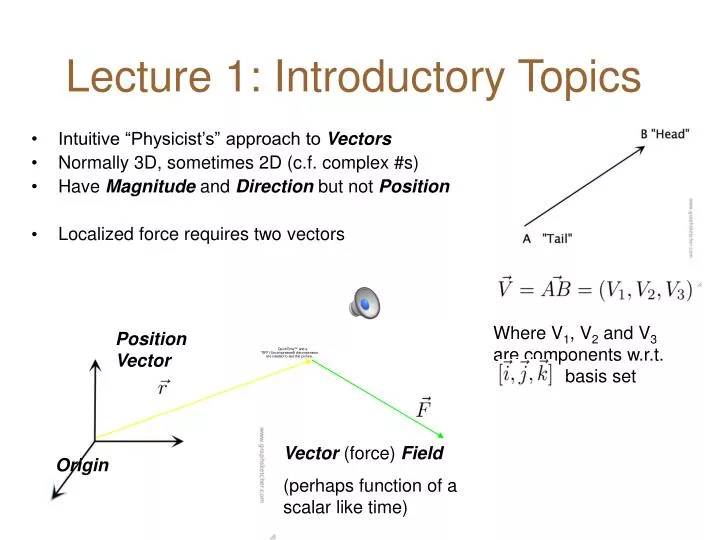
Intuitive “Physicist’s” approach to Vectors Normally 3D, sometimes 2D (c.f. complex #s) Have Magnitude and Direction but not Position Localized force requires two vectors. Lecture 1: Introductory Topics. Where V 1 , V 2 and V 3 are components w.r.t. basis set. Position Vector.

E N D
Intuitive “Physicist’s” approach to Vectors Normally 3D, sometimes 2D (c.f. complex #s) Have Magnitude and Direction but not Position Localized force requires two vectors Lecture 1: Introductory Topics Where V1, V2 and V3 are components w.r.t. basis set Position Vector Vector (force) Field (perhaps function of a scalar like time) Origin
Translation Origin • Parallel transport of a vector; vectors are “moveable” • Vectors are said to be invariant under translation of coordinate axes
RIGHT-HAND RULE ! Rotation • The magnitude (but obviously not direction) of a vector is invariant under rotation of coordinate axes • Convention: “Right-hand corkscrew rule”, positive rotation appears clockwise when viewed parallel (rather than anti-parallel) to the vector; or “Tossed clocks are left-handed”
Inversion P P PR • Inversion of coordinate axes (the parity P transformation) is a reflection of co-ordinate axes in origin • Right-handed set becomes left-handed set • (“Proper”) or Polar vectors are odd, i.e. they reverse in sign under inversion of axes: • Reflections in a plane are equivalent to PR=RP where R is a rotation • Any position vector is an example of a polar vector
Origin Intuitive approach sometimes hazardous 3 3 R1 R2 2 2 6 6 +/2about z +/2about x 3 1 6 2 5 3 • Rotation not in general commutative • Breaks one of the “hidden rules” of vector spaces • Rotation through a finite angle is not a vector +/2about x +/2about z 2 1 6 3 3 5
Or with Earth +/2 +/2 about about z x +/2 +/2 about about x z
Differentiation and integration of vectors • Integration w.r.t. scalar is inverse operation remembering that the integral, and constant of integration, has same nature (vector) as the integrand • From polar vector we get a family of polar vectors
Small rotations as vectors About z then y About y then z IFF angles small, end up at the same place, so is a vector as is angular velocity
Or with Earth Rotating Earth from Oxford to Cambridge: ignoring the non-sphericity of the Earth, we’d still end up on Parker’s Piece regardless of the order of the rotations!
Pseudovectors • Parity transformation (inversion of coordinate axes) leaves unchanged • is even: • Example of an axial vector or pseudovector • Note that any reflection operation (e.g. in xy plane) changes from a right-handed set to a left- handed set • Cross-product generates axial from polar vectors: • [Polar] = [Axial] x [Polar]: • Hence torque, angular momentum,angular velocity and magnetic field are all axial vectors
Vector areas • Define scalar area • Direction perpendicular to S with a RH rule to assign unique direction • Component of in a direction is projected area seen in that direction • Area is a pseudovector • Break into many small joined planes “OUTSIDE” Project onto yz,xz,xy planes “INSIDE” Projected area Angle between normal to the surface and vector (0,0,1) Care with signs! Or something much more crinkled
Scalar Fields • Assigns a scalar (single number) to each point, possibly as a function of other scalars like time: e.g. 2D function like height • For 2D scalar fields chose between using 3rd dimension to represent value (e.g. relief mapfor height) of function or contour map(join points of constant h). • In 3D, with temperature or other scalar; contour surfaces
Vector Fields 2D • Assigns a single vector (in 2D, 2 numbers; in 3D, 3 numbers) to each point, possibly as functions of other scalars like time • Examples: velocity field of a fluid, electric and magnetic fields