Download
1 / 41
440 likes | 756 Views
On Free Mechanical Vibrations. As derived in section 4.1( following Newton’s 2nd law of motion and the Hooke’s law), the D.E. for the mass-spring oscillator is given by:. In the simplest case, when b = 0, and F e = 0, i.e. Undamped, free vibration, we can rewrite the D.E:. As .

E N D
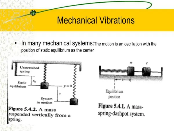
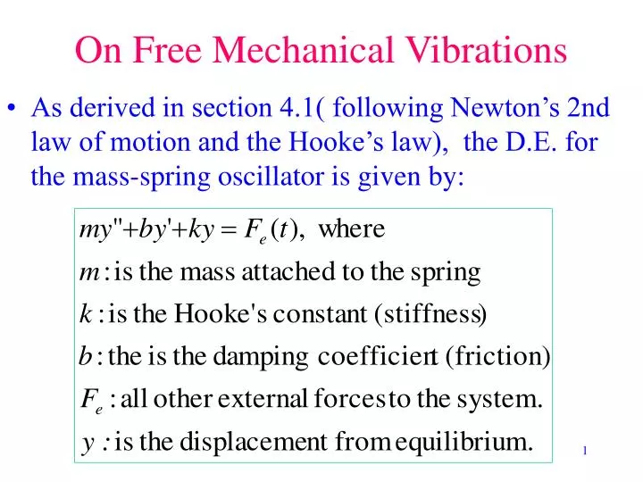
On Free Mechanical Vibrations As derived in section 4.1( following Newton’s 2nd law of motion and the Hooke’s law), the D.E. for the mass-spring oscillator is given by:
In the simplest case, when b = 0, and Fe = 0, i.e. Undamped, free vibration, we can rewrite the D.E: As
When b 0, but Fe = 0, we have damping on free vibrations. The D. E. in this case is:
Case II: Overdamped Motion (b2 > 4mk) In this case, we have two distinct real roots, r1 & r2. Clearly both are negative, hence a general solution: One local max One local min No local max or min
Case III: Critically Damped Motion (b2 = 4mk) We have repeated root -b/2m. Thus the a general solution is:
Example The motion of a mass-spring system with damping is governed by This is exercise problem 4, p239. Find the equation of motion and sketch its graph for b = 10, 16, and 20.
1. b = 10: we have m = 1, k = 64, and b2 - 4mk = 100 - 4(64) = - 156, implies = (39)1/2 . Thus the solution to the I.V.P. is Solution.
When b = 16, b2 - 4mk = 0, we have repeated root -8, thus the solution to the I.V.P is y 1 t
r1 = - 4 and r2 = -16, the solution to the I.V.P. is: When b = 20, b2 - 4mk = 64, thus two distinct real roots are y 1 t 1
with the following D. E. Next we consider forced vibrations
We know a solution to the above equation has the form where: In fact, we have
Thus in the case 0 < b 2 < 4mk (underdamped), a general solution has the form:
Consider the following interconnected fluid tanks Introduction B A 8 L/min Y(t) X(t) 6 L/min 24 L 24 L 6 L/min X(0)= a Y(0)= b 2 L/min
Suppose both tanks, each holding 24 liters of a brine solution, are interconnected by pipes as shown . Fresh water flows into tank A at a rate of 6 L/min, and fluid is drained out of tank B at the same rate; also 8 L/min of fluid are pumped from tank A to tank B, and 2 L/min from tank B to tank A. The liquids inside each tank are kept well stirred, so that each mixture is homogeneous. If initially tank A contains a kg of salt and tank B contains b kg of salt, determine the mass of salt in each tanks at any time t > 0.
Set up the differential equations For tank A, we have: and for tank B, we have
We have the following 2nd order Initial Value Problem: Let us make substitutions: Then the equation becomes: On the other hand, suppose
Thus a 2nd order equation is equivalent to a system of 1st order equations in two unknowns. A system of first order equations
Let us consider an example: solve the system General Method of Solving System of equations: is the Elimination Method.
We want to solve these two equations simultaneously, i.e. find two functions x(t) and y(t) which will satisfy the given equations simultaneously There are many ways to solve such a system. One method is the following: let D = d/dt, then the system can be rewritten as:
(D - 3)[x] + 4y = 1, …..(*)-4x + (D + 7)[y]= 10t .…(**) The expression 4(*) + (D - 3)(**) yields: {16 + (D - 3)(D + 7)}[y] = 4+(D - 3)(10t), or (D2 + 4D - 5)[y] =14 - 30t. This is just a 2nd order nonhomogeneous equation. The corresponding auxiliary equation is r2 + 4r - 5 = 0, which has two solution r = -5, and r = 1, thus yh = c1e -5t + c2 e t. And the general solution is y = c1e -5t + c2 e t + 6t + 2. To find x(t), we can use (**).
To find x(t), we solve the 2nd eq.Y(t) = 4x(t) - 7y(t)+ 10t for x(t), We obtain:
Generalization Let L1, L2, L3, and L4 denote linear differential operators with constant coefficients, they are polynomials in D. We consider the 2x2 general system of equations:
Rewrite the system in operator form: (D2 - 1)[x] + (D + 1)[y] = -1, .……..(3) (D - 1)[x] + D[y] = t2 ……………...(4) To eliminate y, we use D(3) - (D + 1)(4) ; which yields: {D(D2 - 1) - (D + 1)(D - 1)}[x] = -2t - t2. Or {(D(D2 - 1) - (D2 - 1)}[x] = -2t - t2. Or {(D - 1)(D2 - 1)}[x] = -2t - t2. Example:
Which implies r = 1, 1, -1. Hence the general solution to the homogeneous equation is xh = c1e t + c2te t + c3e -t. Since g(t) = -2t - t2, we shall try a particular solution of the form : xp = At2 + Bt + C, we find A = -1, B = -4, C = -6, The general solution is x = xh + xp. The auxiliary equation for the corresponding homogeneous eq. is (r - 1)(r2 - 1) = 0
Which implies y = (D - D2)[x] -1 - t2. To find y, note that (3) - (4) yields : (D2 - D)[x] + y = -1 - t2.
This is simply a mapping of functions to functions This is an integral operator. Chapter 7: Laplace Transforms L F f f F
Definition: Let f(t) be a function on [0, ). The Laplace transform of f is the function F defined by the integral The domain of F(s) is all values of s for which the integral (*) exists. F is also denoted by L{f}. More precisely
Example 1. Consider f(t) = 1, for all t > 0. We have
Other examples, 2. Exponential function f(t) = e t . 3. Sine and Cosine functions say: f(t) = sin ßt, 4. Piecewise continuous (these are functions with finite number of jump discontinuities).
Example 4, P.375 A function is piecewise continuous on [0, ), if it is piecewise continuous on [0,N] for any N > 0.
Function ofExponential Order Definition. A function f(t) is said to be of exponential order if there exist positive constants M and T such that That is the function f(t) grows no faster than a function of the form For example: f(t) = e 3t cos 2t, is of order = 3.
Existence Theorem of Laplace Transform. Theorem: If f(t) is piecewise continuous on [0, ) and of exponential order , then L{f}(s) exists for all s > . Proof.We shall show that the improper integral converges for s > . This can be seen easily, because [0, ) = [0, T] [ T, ). We only need to show that integral exists on [ T, ).
A table of Laplace Transforms can be found on P. 380 Remarks: 1. Laplace Transform is a linear operator. i.e. If the Laplace transforms of f1 and f2 both exist for s > , then we have L{c1 f1 + c2 f2} = c1L{f1 } + c2L{f2 } for any constants c1 and c2 . 2. Laplace Transform converts differentiation into multiplication by “s”.
Properties of Laplace Transform Recall : Proof.
1. e -2t sin 2t + e 3t t2. 2. t n. 3. t sin (bt). Some Examples.