Download
1 / 25
250 likes | 408 Views
Parallel Computers. References: [1] - [4] given below; [5] & [6] given on slide 14. Chapter 1, “Parallel Programming ” by Wilkinson, el. Chapter 1, “Parallel Computation” by Akl Chapter 1-2, “Parallel Computing” by Quinn, 1994

E N D
Parallel Computers • References: [1] - [4] given below; [5] & [6] given on slide 14. • Chapter 1, “Parallel Programming ” by Wilkinson, el. • Chapter 1, “Parallel Computation” by Akl • Chapter 1-2, “Parallel Computing” by Quinn, 1994 • Chapter 2, “Parallel Processing & Parallel Algorithms” by Roosta • Need for Parallelism • Numerical modeling and simulation of scientific and engineering problems. • Solution for problems with deadlines • Command & Control problems like ATC. • Grand Challenge Problems • Sequential solutions may take months or years. • Weather Prediction - Grand Challenge Problem • Atmosphere is divided into 3D cells. • Data such as temperature, pressure, humidity, wind speed and direction, etc. are recorded at regular time-intervals in each cell. • There are about 5108 cells of (1 mile) 3 . • It would take a modern computer over 100 days to perform necessary calculations for 10 day forecast. • Parallel Programming - a viable way to increase computational speed. • Overall problem can be split into parts, each of which are solved by a single processor. Parallel Computers
Ideally, n processors would have n times the computational power of one processor, with each doing 1/nth of the computation. • Such gains in computational power is rare, due to reasons such as • Inability to partition the problem perfectly into n parts of the same computational size. • Necessary data transfer between processors • Necessary synchronizing of processors • Two major styles of partitioning problems • (Job) Control parallel programming • Problem is divided into the different, non-identical tasks that have to be performed. • The tasks are divided among the processors so that their work load is roughly balanced. • This is considered to be coarse grained parallelism. • Data parallel programming • Each processor performs the same computation on different data sets. • Computations do not necessarily have to be synchronous. • This is considered to be fine grained parallelism. Parallel Computers
Shared Memory Multiprocessors (SMPs) • All processors have access to all memory locations . • The processors access memory through some type of interconnection network. • This type of memory access is called uniform memory access (UMA) . • A data parallel programming language, based on a language like FORTRAN or C/C++ may be available. • Alternately, programming using threads is sometimes used. • More programming details will be discussed later. • Difficulty for the SMP architecture to provide fast access to all memory locations result in most SMPs having hierarchial or distributed memory systems. • This type of memory access is called nonuniform memory access (NUMA). • Normally, fast cache is used with NUMA systems to reduce the problem of different memory access time for PEs. • This creates the problem of ensuring that all copies of the same date in different memory locations are identical. • Numerous complex algorithms have been designed for this problem. Parallel Computers
(Message-Passing) Multicomputers • Processors are connected by an interconnection network. • Each processor has a local memory and can only access its own local memory. • Data is passed between processors using messages, as dictated by the program. • Note: If the processors run in SIMD mode (i.e., synchronously), then the movement of the data movements over the network can be synchronous: • Movement of the data can be controlled by program steps. • Much of the message-passing overhead (e.g., routing, hot-spots, headers, etc. can be avoided) • Synchronous parallel computers are not usually included in this group of parallel computers. • A common approach to programming multiprocessors is to use message-passing library routines in addition to conventional sequential programs (e.g., MPI, PVM) • The problem is divided into processes that can be executed concurrently on individual processors. A processor is normally assigned multiple processes. • Multicomputers can be scaled to larger sizes much better than shared memory multiprocessors. Parallel Computers
Multicomputers (cont.) • Programming disadvantages of message-passing • Programmers must make explicit message-passing calls in the code • This is low-level programming and is error prone. • Data is not shared but copied, which increases the total data size. • Data Integrity: difficulty in maintaining correctness of multiple copies of data item. • Programming advantages of message-passing • No problem with simultaneous access to data. • Allows different PCs to operate on the same data independently. • Allows PCs on a network to be easily upgraded when faster processors become available. • Mixed “distributed shared memory” systems • Lots of current interest in a cluster of SMPs. • See David Bader’s or Joseph JaJa’s website • Other mixed systems have been developed. Parallel Computers
Flynn’s Classification Scheme • SISD - single instruction stream, single data stream • Primarily sequential processors • MIMD - multiple instruction stream, multiple data stream. • Includes SMPs and multicomputers • processors are asynchronous, since they can independently execute different programs on different data sets. • Considered by most researchers to contain the most powerful, least restricted computers. • Have very serious message passing (or shared memory) problems that are often ignored when • compared to SIMDs • when computing algorithmic complexity • May be programmed using a multiple programs, multiple data (MPMD) technique. • A common way to program MIMDs is to use a single program, multiple data (SPMD) method • Normal technique when the number of processors are large. • Data Parallel programming style for MIMDs • SIMD: single instruction and multiple data streams. • One instruction stream is broadcast to all processors. Parallel Computers
Flynn’s Taxonomy (cont.) • SIMD (cont.) • Each processor (also called a processing element or PE) is very simplistic and is essentially an ALU; • PEs do not store a copy of the program nor have a program control unit. • Individual processors can be inhibited from participating in an instruction (based on a data test). • All active processor executes the same instruction synchronously, but on different data (from their own local memory). • The data items form an array and an instruction can act on the complete array in one cycle. • MISD - Multiple Instruction streams, single data stream. • This category is not used very often. • Some include pipelined architectures in this category. Parallel Computers
Interconnection Network Terminology • A link is the connection between two nodes. • A switch that enables packets to be routed through the node to other nodes without disturbing the processor is assumed. • The link between two nodes can be either bidirectional or use two directional links . • Either one wire to carry one bit or parallel wires (one wire for each bit in word) can be used. • The above choices do not have a major impact on the concepts presented in this course. • The diameter is the minimal number of links between the two farthest nodes in the network. • The diameter of a network gives the maximal distance a single message may have to travel. • The bisection width of a network is the number of links that must be cut to divide the network of n PEs into two (almost) equal parts, n/2 and n/2. Parallel Computers
Interconnection Network Terminology (cont.) • The below terminology is given in [1] and will be occasionally needed (e.g., see “Communications” discussion starting on page 16). • The bandwidth is the number of bits that can be transmitted in unit time (i.e., bits per second). • The network latency is the time required to transfer a message through the network. • The communication latency is the total time required to send a message, including software overhead and interface delay. • The message latency or startup time is the time required to send a zero-length message. • Software and hardware overhead, such as • finding a route • packing and unpacking the message Parallel Computers
Interconnection Network Examples • References: 1-4 discuss these network examples, but reference 3 (Quinn) is particularly good. • Completely Connected Network • Each of n nodes has a link to every other node. • Requires n(n-1)/2 links • Impractical, unless very few processors • Line/Ring Network • A line consists of a row of n nodes, with connection to adjacent nodes. • Called a ring when a link is added to connect the two end nodes of a line. • The line/ring networks have many applications. • Diameter of a line is n-1 and of a ring is n/2. • Minimal distance, deadlock-free parallel routing algorithm: Go shorter of left or right. Parallel Computers
Interconnection Network Examples (cont) • The Mesh Interconnection Network • Each node in a 2D mesh is connected to all four of its nearest neighbors. • The diameter of a n n mesh is 2(n - 1) • Has a minimal distance, deadlock-free parallel routing algorithm: First route message up or down and then right or left to its destination. • If the horizonal and vertical ends of a mesh to the opposite sides, the network is called a torus. • Meshes have been used more on actual computers than any other network. • A 3D mesh is a generalization of a 2D mesh and has been used in several computers. • The fact that 2D and 3D meshes model physical space make them useful for many scientific and engineering problems. Parallel Computers
Interconnection Network Examples (cont) • Binary Tree Network • A binary tree network is normally assumed to be a complete binary tree. • It has a root node, and each interior node has two links connecting it to nodes in the level below it. • The height of the tree is lg n and its diameter is 2 lg n . • In an m-ary tree,each interior node is connected to m nodes on the level below it. • The tree is particularly useful for divide-and-conquer algorithms. • Unfortunately, the bisection width of a tree is 1 and the communication traffic increases near the root, which can be a bottleneck. • In fat tree networks, the number of links is increased as the links get closer to the root. • Thinking Machines’ CM5 computer used a 4-ary fat tree network. Parallel Computers
Interconnection Network Examples (cont) • Hypercube Network • A 0-dimensional hypercube consists of one node. • Recursively, a d-dimensional hypercube consists of two (d-1) dimensional hypercubes, with the corresponding nodes of the two (d-1) hypercubes linked. • Each node in a d-dimensional hypercube has d links. • Each node in a hypercube has a d-bit binary address. • Two nodes are connected if and only if their binary address differs by one bit. • A hypercube has n = 2d PEs • Advantages of the hypercube include • its low diameter of lg(n) or d • its large bisection width of n/2 • its regular structure. • An important practical disadvantage of the hypercube is that the number of links per node increases as the number of processors increase. • Large hypercubes are difficult to implement. • Usually overcome by increasing nodes by replacing each node with a ring of nodes. • Has a “minimal distance, deadlock-free parallel routing” algorithm called e-cube routing: • At each step, the current address and the destination address are compared. • Each message is sent to the node whose address is obtained by flipping the leftmost digit of current address where two addresses differ. Parallel Computers
Embedding • References: [1, Wilkinson] and [3, Quinn]. Quinn is the best of 1-4, but it does not cover a few topics. Also, two additional references should be added to our previous list. Reference [5] below has a short coverage of embeddings and [6] has an encyclopedic coverage of many topics including embeddings. • [5] “Introduction to Parallel Computing”, Vipin Kumar, Grama, Gupta, & Karypis, 1994, Benjamin/Cumming, ISBN 0-8053-3170-0. • [6] “Introduction to Parallel Algorithm & Architectures”, F. Thomson Leighton, 1992, Morgan Kaufmann. • An embedding is a 1-1 function (also called a mapping) that specifies how the nodes of domain network can be mapped into a range network. • Each node in range network is the target of at most one node in the domain network, unless specified otherwise. • The domain network should be as large as possible with respect to the range network. • Reference 1 calls an embedding perfect if each link in the domain network corresponds under the mapping to a link in the range network. • Nearest neighbors are preserved by mapping. • A perfect embedding of a ring onto a torus is shown in Fig. 1.15. • A perfect embedding of a mesh/torus in a hypercube is given in Figure 1.16 • Uses Gray code along each mesh dimension. Parallel Computers
The dilation of an embedding is the maximum number of links in the range network corresponding to one link in the domain network (i.e., its ‘stretch’) • Perfect embeddings have a dilation of 1. • Embedding of binary trees in other networks are used in Ch. 3-4 in [1] for broadcasts and reductions. • Some results on binary trees embeddings follow. • Theorem: A complete binary tree of height greater than 4 can not be embedded in a 2-D mesh with a dilation of 1. (Quinn, 1994, pg135) • Hmwk Problem: A dilation-2 embedding of a binary tree of height 4 is given in [1, Fig. 1.17]. Find a dilation-1 embedding of this binary tree. • Theorem: There exists an embedding of a complete binary tree of height n into a 2D mesh with dilation n/2. • Theorem: A complete binary tree of height n has a dilation-2 embedding in a hypercube of dimension n+1 for all n > 1. • Note: Network embeddings allow algorithms for the domain network to be transferred to the target nodes of the range network. • Warning: In [1], the authors often use the words “onto” and “into” incorrectly, as an embedding is technically a mapping (i.e., a 1-1 function). Parallel Computers
Communication Methods • References: [1], [5], and [6]. Coverage here follows [1]. References [5] and [6] are older but more highly regarded and better known references. • Two basic ways of transferring messages from source to destination. • Circuit switching • Establishing a path and allowing the entire message to transfer uninterrupted. • Similar to telephone connection that is held until the end of the call. • Links are not available to other messages until the transfer is complete. • Latency (or message transfer time): If the length of control packet sent to establish path is small wrt (with respect to) the message length, the latency is essentially • the constant L/B, where L is message length and B is bandwidth. • packet switching • Message is divided into “packets” of information • Each packet includes source and destination addresses. • Packets can not exceed a fixed, maximum size (e.g., 1000 byte). • A packet is stored in a node in a buffer until it can move to the next node. Parallel Computers
Communications (cont) • At each node, the designation information is looked at and used to select which node to forward the packet to. • Routing algorithms (often probabilistic) are used to avoid hot spots and to minimize traffic jams. • Significant latency is created by storing each packet in each node it reaches. • Latency increases linearly with the length of the route. • Store-and-forward packet switching is the name used to describe preceding packet switching. • Virtual cut-through package switching can be used to reduce the latency. • Allows packet to pass through a node without being stored, if the outgoing link is available. • If complete path is available, a message can immediately move from source to destination.. • Wormhole Routing alternate to store-and-forward packet routing • A message is divided into small units called flits (flow control units). • flits are 1-2 bytes in size. • can be transferred in parallel on links with multiple wires. • Only head of flit is initially transferred when the next link becomes available. Parallel Computers
Communications (cont) • As each flit moves forward, the next flit can move forward. • The entire path must be reserved for a message as these packets pull each other along (like cars of a train). • Request/acknowledge bit messages are required to coordinate these pull-along moves. (see [1]) • The complete path must be reserved, as these flits are linked together. • Latency: If the head of the flit is very small compared to the length of the message, then the latency is essentially the constant L/B, with L the message length and B the link bandwidth. • Deadlock • Routing algorithms needed to find a path between the nodes. • Adaptive routing algorithms choose different paths, depending on traffic conditions. • Livelock is a deadlock-type situation where a packet continues to go around the network, without ever reaching its destination. • Deadlock: No packet can be forwarded because they are blocked by other stored packets waiting to be forwarded. • Input/Output: A significant problem on all parallel computers. Parallel Computers
Metrics for Evaluating Parallelism • References: All references cover most topics in this section and have useful information not contained in others. Ref. [2, Akl] includes new research and is the main reference used, although others (esp. [3, Quinn] and [1, Wilkinson]) are also used. • Granularity: Amount of computation done between communication or synchronization steps and is ranked as fine, intermediate, and coarse. • SIMDs are built for efficient communications and handle fine-grained solutions well. • SMPs or message passing MIMDS handle communications less efficiently than SIMDs but more efficiently than clusters and can handle intermediate-grained solutions well. • Cluster of Workstations or distributed systems have slower communications among processors and is appropriate for coarse grain applications. • For asynchronous computations, increasing the granularity • reduces expensive communications • reduces costs of process creation • but reduces the nr of concurrent processes • Speedup • A measure of the increase in running time due to parallelism. • Based on running times, S(n) = ts/tp , where • ts is the execution time on a single processor, using the fastest known sequential algorithm Parallel Computers
Parallel Metrics (cont) where • tp is the execution time using a parallel processor. • In theoretical analysis, S(n) = ts/tpwhere • tsis the worst case running time for of the fastest known sequential algorithm for the problem • tp is the worst case running time of the parallel algorithm using n PEs. • False Claim: The maximum speedup for a parallel computer with n PEs is n (called linear speedup). Proof for “traditional problems” is: • Assume computation is divided perfectly into n processes of equal duration. • Assume no overhead is incurred • Then, a optimal parallel running time of n is obtained • This yields an absolute maximal running time of ts /n. • Then S(n) = ts /(ts /n) = n. • Normally, the speedup is much less than n, as • above assumptions usually do not occur. • Usually some parts of programs are sequential and only one PE is active Parallel Computers
Parallel Metrics (cont) • During parts of the execution, some PEs are waiting for data to be received or to send messages. • Superlinear speedup (i.e., when S(n) > n): • Most texts besides [2,3] states that while this can happen, it is rare and due to reasons such as • extra memory in parallel system. • a sub-optimal sequential algorithm used. • luck, in case of algorithm that has a random aspect in its design (e.g., random selection) • Selim Akl has shown that for some less standard problems, superlinearity will occur: • Some problems can not be solved without use of parallel computation. • Some problems are natural to solve using parallelism and sequential solutions are inefficient. • The final chapter of his textbook and several journal papers have been written to establish these claims are valid, but it may still be a long time before they are fully accepted. • Superlinearity has been a hotly debated topic for too long to be accepted quickly. Parallel Computers
Amdahl’s Law • Assumes that the speedup is not superliner; i.e., S(n) = ts/ tp n • Assumption only valid for traditional problems. • By Figure 1.29 in [1] (or slide #40), if f denotes the fraction of the computation that must be sequential, tp f ts + (1-f) ts /n • Substituting above values into the above equation for S(n) and simplifying (see slide #41 or book) yields • Amdahl’s “law”: S(n) 1/f, where f is as above. • See Slide #41 or Fig. 1.30 for related details. • Note that S(n) never exceed 1/f and approaches 1/f as n increases. • Example: If only 5% of the computation is serial, the maximum speedup is 20, no matter how many processors are used. • Observations: Amdahl’s law limitations to parallelism: • For a long time, Amdahl’s law was viewed as a severe limit to the usefulness of parallelism. Parallel Computers
Primary Reason Amdahl’s Law is “flawed”. • Gustafon’s Law: The proportion of the computations that are sequential normally decreases as the problem size increases. • Other flaws in Amdahl’s Law: • The argument focuses on the steps in a particular algorithm • Assumes an algorithm with ‘more parallelism’ does not exist. • Amdahl’s law applies only to standard problems were superlinearity doesn’t occurs. • For more details on superlinearity, see [2] “Parallel Computation: Models and Methods”, Selim Akl, pgs 14-20 (Speedup Folklore Theorem) and Chapter 12. Parallel Computers
More Metrics for Parallelism • Efficiency is defined by • Efficiency give the percentage of full utilization of parallel processors on computation, assuming a speedup of n is the best possible. • Cost: The cost of a parallel algorithm or parallel execution is defined by Cost = (running time) (Nr. of PEs) = tp n • Observe that • Cost allows the “goodness” of a parallel algorithm to be compared to a sequential algorithm • Compare cost of parallel algorithm to running time of sequential algorithm • If a sequential algorithm is executed in parallel and each PE does 1/n of the work in 1/n of the sequential running time, then the parallel cost is the same as the sequential running time. Parallel Computers
More Metrics (cont.) • Cost-Optimal Parallel Algorithm: A parallel algorithm for a problem is said to be cost-optimal if its cost is proportional to the running time of an optimal sequential algorithm for the same problem. • By proportional, we means that cost = tp n = k ts where k is a constant. (See pg 67 of [1]). • Equivalently, a parallel algorithm is optimal if parallel cost = O(f(t)), where f(t) is the running time of an optimal sequential algorithm. • In cases where no optimal sequential algorithm is known, then the “fastest known” sequential algorithm is often used instead. • Also, see pg 67 of [1, Wilkinson]. Parallel Computers