Download

1 / 35
350 likes | 508 Views
Volume, Volatility and Stock Return on the Romanian Stock Market Dissertation paper. MSc Student: Valentin STANESCU Supervisor: Professor Moisa ALTAR. Previous research about volume. Lamorieux and Laplace (1991) Gallant, Rossi and Tauchen (1992) Karpoff (1987)

E N D
Volume, Volatility and Stock Returnon the Romanian Stock MarketDissertation paper MSc Student: Valentin STANESCU Supervisor: Professor Moisa ALTAR
Previous research about volume • Lamorieux and Laplace (1991) • Gallant, Rossi and Tauchen (1992) • Karpoff (1987) • contemporaneous stock price-volume relation • Rogalsky (1978), Smirlock and Starks (1988), Jain and Joh (1988) and Antoniewicz (1992) • traditional Granger causality tests • Baek and Brock (1992), Hiemstra and Jones (1993,1994) • nonlinear Granger tests
The Data • Estimation and training: • 953 observations 16/6/1997 until 2/08/2001 • test data: • 200 from 3/08/2001 until 1/7/2002 • Eliminated non trading days • Volume = no. of shares • Price = closing price • Volume precedes price
Modeling the series • Unit root in price => return. Volume is I(0).
Detrended volume Long term analysis is not a goal of the paper Short term trend might contain relevant information
GARCH equation for the return Note the persistence in volatility
Zooming in... Notice how the volume spikes up when the volatility increases Sometimes the reaction of the volume follows the increase of the volatility (continuous line) but sometimes it precedes the turbulent period (dotted line). Is there a link between the two?
Linear Granger tests, volume vs variance and vs return Volume causes the variance but there is no linear relation to the return
Explanations for causality • the sequential information arrival models • Copenland (1976), Jennings, Starks and Fellingham (1981) • tax and non-tax related motives for trading • Lakonishok and Schmidt (1989) • mixture of distributions models • Clark (1973) and Epps and Epps (1976) • noise trader models • not based on fundamentals • stock returns are positively autocorrelated in the short run, but negatively autocorrelated in the long run
VAR of Volume and Variance Lags of variance and volume explain 80% of the variance
Volume in variance equation There is no more persistence in volatility
Dummies for volume Significant coefficients but small and irrelevant R squared.
Implications • return variance was slowly adjusted because of the persistence, now it is volume dependent • mean return is still set to zero because of a lack of a better prediction • the volume has a AR mean equation which leads to a predictable value, unlike the return’s • return variance is forecasted instead of adapted • Applications • Risk management • Option strategies • Delta hedged portfolio • Other strategies involving the volatility
Granger causality • General: • Time series (linear): • Non-linear: • is not detected by a linear Granger test • let:
Non-linear causality • Testable implication: • we note:
Statistic • Statistic: • Estimated:
Estimation • Variance: • d(n) = { 1/C2(Lx,Ly,e,n) , -C1(m+Lx,Ly,e,n)/C22(Lx,Ly,e,n) , -1/C4(Lx,e,n) , C3(m+Lx,e,n)/C42(Lx,e,n) }
Nonlinear Granger test • Linear VAR residuals of simple GARCH filtered returns and of volume factor GARCH filtered returns, scaled to share a common standard deviation of 1 and thus a common scale factor e. • Heuristic approach to find “the needle in the hay stack”. • 10% statistically significant causality from volume to return in both cases for T=952, m=1, Lx=8, Ly=6 and e=0.3 • Insignificant results for a relation running from returns to volume • Problems: • how to determine the remaining relations? • is the relation always present?
Fuzzy logic and neural networks • Classic algebra • Patched function • subsets • noise resistant • triangles are probabilities • Explicit rules • Internal significance test
The internal mechanism • The fuzzy logic neural network does not extract all the possible rules and assign probabilities to them, instead it tries to • increase or decrease the degree of a fuzzy variable, the number of sets, the location of the set separator, the links between the subnetworks and the variables and the probabilities. • The degree of a variable is the number of sets it can belong to • The number of sets is adjusted and the center of all the sets is moved to minimize their cumulated distance to the observations • For each required output a network is created and they are trained simultaneously • By changing the connections between the inputs and the subnetworks of a network an input may be found to be irrelevant to a certain output.
The information set and targets • The information set considers the parameters where the nonlinear Granger test indicated causality: • eight lags of the return, absolute return, and squared return • current and six lags of volume • alternate set that included the price • Targets: • current return, absolute return, squared return • buy decision, buy/sell decision • volume (adjusted information set)
Results • Failure...to model: • current return • buy decision • buy/sell decision • Weird results for price => discarded • Success: • absolute returns • squared returns • volume • All the variables had a degree of two showing that they belonged to just two subsets.
Squared return • Relevant information: • volume and 1 lag squared return, divided in two subsets • Rules extracted • if volume is small then squared return will almost surely be small • if volume is large then squared return will almost surely be large • This confirms the econometric results in which volume was linked to volatility as in Lamourieux and Laplace (1991) and Clark’s models.
Absolute returns • Relevant information: • 1 lag absolute return and volume, both with two subsets • Rules extracted: • if volume is small then absolute return will be almost surely small • if volume is large then absolute return will be small with 32% probability or large with 68% probability • if the 1 lag absolute return is small then the current absolute return will be small with 72% probability or large with 28% probability • if the 1 lag absolute return is large then the current absolute return will almost surely be large • Rule 1 and the second part of rule 2 show a positive correlation between volume and absolute return but the first part indicates the possibility of a negative correlation. This result is consistent with the sequential information arrival models of Copeland (1976) and Jennings, Starks and Fellingham (1981).
Volume • Relevant information: two lags of volume • Rules extracted: • if the first lagged volume is small then the current volume will almost surely be small • if the first lagged volume is large then the current volume will almost surely be large • if the second lag is small then current value will be small with 77% probability or large with 23% probability • if the second lag is large then current value will be small with 12% probability or large with 88% probability • These rules only confirm the autoregressive in mean, heteroskedastic, with persistence in variance estimated TARCH model, but only the first two lags were deemed relevant. It may be that the volume depends on other factors like the speed of information flow from Clark’s model.
Evaluating the network • Just for the absolute and squared returns, and volume • The network performs its own internal tests when deciding whether to drop a rule, a subnetwork or make other adjustments. If the new configuration is better at explaining the data then the components added were significant and those removed had little explanatory power. When evaluating the network on the last 200 observations these internal mechanisms showed that the network performed well on data not presented to it in the training stages.
Conclusions and remarks • In line with the empirical results obtained in the literature on the stock price-volume relation by indicating the presence of a nonlinear Granger causality between closing prices and volume. • Suggests that researchers should consider nonlinear theoretical mechanisms and empirical regularities when devising and evaluating models of the joint dynamics of stock prices and trading volume. Or the fact that they could be related through different functions for each subset. • No guidance regarding the source or form of the nonlinear dependence. • The relation between return, variance and volume was partially modeled but the process governing the volume could not be modeled better than using a GARCH model. This could be an interesting goal for future research.
References • Andersen, T. (1992), Return volatility and trading volume in financial markets: An information flow interpretation of stochastic volatility, Working paper, Northwestern University • Antoniewicz, R. (1992), A causal relationship between stock returns and volume, Working paper, Federal Reserve Board • Baek, E. and W.Brock (1992), A general test for nonlinear Granger causality: Bivariate model, Working paper, Iowa State University and University of Wisconsin, Madison • Berndt, E., B. Hall, and J. Hausman (1974), Estimation and inference in nonlinear structural models, Annals of Economic and Social Measurement 3, 653-665 • Brock, W., D. Hsieh, and B. LeBaron (1991), A Test of Nonlinear Dynamics, Chaos, and Instability: Statistical Theory and Economic Evidence, MIT Press, Cambridge. • Campbell, J., S. Grossman, and J. Wang (1993), Trading volume and serial correlation in stock returns, Quarterly Journal of Economics 108, 905-939 • Clark, P. (1973), A subordinated stochastic process model with finite variances for speculative prices, Econometrica 41, 135-155 • Copeland T. (1976), A model of asset trading under the assumption of sequential information arrival, Journal of Finance 31, 135-155 • Dikerson, J, and B. Kosko (1996), Fuzzy function approximation with ellipsoidal rules, IEEE Transations on systems, man, and cybernetics – part B: Cybernetics, vol 26, no. 4 • Duffe, G. (1992), Trading volume and return reversals, Working paper, Federal Reserve Board
References • Engle, R. (1982) Autoregressive conditional heteroskedasticity with estimates of the variance of the United Kingdom inflation, Econometrica 50, 987-1007 • Epps, T., and M. Epps (1976), The stochastic dependence of security price changes and transaction volumes: Implications for the mixture of distributions hypothesis, Econometrica 44, 305-321 • Fama, E., and K. French (1988), Permanent and temporary components of stock prices, Journal of Political Economy 96, 246-273 • Gallant, R., P. Rossi, and G. Tauchen (1992a), Stock prices and volume, Review of Financial Studies 5, 199-242 • (1992b), Nonlinear dynamic structures, Econometrica 61, 871-907 • Hiemstra, C., and J. Jones (1992), Detection and description of linear and nonlinear dependence in daily Dow Jones stock returns and NYSE trading volume, Working paper, University of Strathclyde and Securities and Exchange Commission • Hinich, M. and D. Patterson, (1985), Evidence of nonlinearity in stock returns, Journal of Business and Economic Statistics 3, 69-77 • Hsieh, D. (1991), Chaos and nonlinear dynamics: Application to financial markets, Journal of Finance 46, 1839-1877 • Jain, P. and G. Joh (1988), The dependence between hourly prices and trading volume, Journal of Financial and Quantitative Analysis 23, 269-283
References • Jennings, R., L. Starks, and J. Fellingham (1981), An equilibrium model of asset trading with sequential information arrival, Journal of Finance 36, 143-161 • Karpoff, J. (1987), The relation between price changes and trading volume: A survey, Journal of Financial and Quantitative Analysis 22, 109-126 • Kosko, B. (1988), Bidirectional Associative Memory, IEEE Transactions on systems, man and cybernetics, vol. 18, no. 1 • Kosko, B. (1990a), Unsupervised learning in noise, IEEE Transactions on neural networks, vol. 1, no. 1 • Kosko, B., and S. Mitaim (1997), Adaptive stochastic resonance, IEEE Transactions on neural networks • Lakonishok, J., and S. Smidt (1989), Past price changes and current trading volume, The Journal of Portfolio Management 15, 18-24 • Lamoureux, C., and W. Lastrapes (1990), Heteroskedasticity in stock return data: Volume versus GARCH effects, Journal of Finance 45, 221-229 • Scheinkman, J., and B. LeBaron (1989), Nonlinear dynamics and stock returns, Journal of Business 62, 311-337 • White, H. (1980), A heteroscedasticity-consistent covariance matrix estimator and a direct test for heteroskedasticity, Econometrica 48, 817-838