A linear time approximation scheme for Euclidean TSP

1. A linear time approximation scheme for Euclidean TSP • YairBartalHebrew University • Lee-Ad GottliebAriel University TexPoint fonts used in EMF. Read the TexPoint manual before you delete this box.: AAAA

2. Traveling salesman problem • Definition: Given a set of cities (points) find a minimum tour that visits each point • Classic, well-studied NP-hard problem • [Karp ‘72; Papadimitriou, Vempala ‘06] • Mentioned in a handbook from 1832! • Common benchmark for optimization methods • Many books devoted to TSP • Other variants • Closed tour • Multiple tours • Etc… Optimal tour

3. Euclidean TSP • SanjeevArora [A ‘98] and Joe Mitchell [M ‘99] : Euclidean TSP with fixed dimension admits a PTAS • (1+Ɛ)-approximate tour • In time n(log n)Ɛ-Ỡ(d) • Easy extension to other norms • They were awarded the 2010 Gödel Prize for this discovery 3

4. Euclidean TSP • Shortly after Arora’s PTAS appeared, Rao-Smith improved its runtime. • Arora: n(logn)Ɛ-Ỡ(d) • Rao-Smith: 2Ɛ-Ỡ(d)n + 2Ỡ(d)nlog n • Rao-Smith: Is linear time possible? • Question reiterated by Chan ‘08, Borradaile-Epstein ’12. 4

5. Euclidean TSP • Shortly after Arora’s PTAS appeared, Rao-Smith improved its runtime • Arora: n(logn)Ɛ-Ỡ(d) • Rao-Smith: 2Ɛ-Ỡ(d)n + 2Ỡ(d)nlog n • Rao-Smith: Is linear time possible? • Question reiterated by Chan ‘08, Borradaile-Epstein ’12. • Computational model • Cell-probe model: Ω(nlogn) bound via sorting [Das, Kapoor, Smid ‘97] • What about real/integer RAM? • This paper: Linear time approximation scheme in integer RAM model • Runtime: 2Ɛ-Ỡ(d)n • Assume: integer coordinates in range [0,O(n)] 5

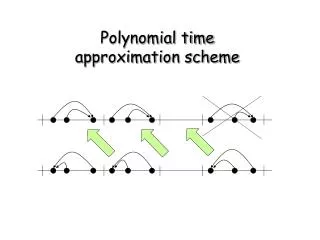
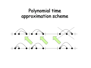
6. Talk Outline • Step 1: Preliminaries • Outline Arora’salorithm: Quadtree • Rao-Smith improvement: Spanner • Step 2: Present our algorithm • Faster implementation of Rao-SmithSparse decomposition

7. Arora’s Quadtree • Random quadtree Min distance 1

8. Arora’s Quadtree • Random quadtree 4-level 24=16 Random offset

9. Arora’s Quadtree • Random quadtree 3-level 23=8

10. Arora’s Quadtree • Random quadtree 2-level 22=4

11. Arora’s Quadtree • Random quadtree 1-level 21=2

12. Arora’s Quadtree • Random quadtree 0-level 20=1

13. Arora’s Quadtree • Definition: A tour is (m,r)-light on a quadtree if it enters all cells (clusters) • At most r times • Only via m pre-defined portals

14. Arora’s Quadtree • Given quadtree Q • The best (m,r)-light tour on Q can be computed exactly in mO(r)+nlogn time • Via simple dynamic programming • Arora showed that a good (m,r)-light tour always exists

15. Arora’s Quadtree • Existence of a good (m,r)-light tour • Modify OPT (unknown) • Achieve (m,r)-light tour close to OPT • Step 1: Move cut edges to portals • Step 2: Reduce the number of crossings (patching)

16. Euclidean TSP • How can Arora’s runtime be improved? • Rao-Smith: Spanners reduce portals • Reduce number of portals • Arora: m = logO(d)n portals • Rao & Smith: m = Ɛ-O(d) portals • Recall that runtime is ~ mO(r) • r = Ɛ-O(d) • Arora: n(log n)Ɛ-Ỡ(d) • Rao-Smith: 2Ɛ-Ỡ(d)n + 2Ỡ(d)nlog n 16

17. Spanner • A spanner is a subgraph with favorable properties • Stretch • Weight (lightness) • Euclidean spaces admit good spanners • Weight ~ O(MST) ~ O(OPT) • (1+Ɛ)-stretch • Best spanner tour is close to OPT G H 1 2 2 1 1 1 1

18. Spanner • A spanner is a subgraph with favorable properties • Stretch • Weight (lightness) • Euclidean spaces admit good spanners • Weight ~ O(MST) ~ O(OPT) • (1+Ɛ)-stretch • Best spanner tour is close to OPT G H 1 2 2 1 1 1 1

19. Spanner • Arora: required many portals for unknown tour • Rao-Smith: Spanner determines portals

20. Linear time • Main tools employed by Rao-Smith • Quadtree • light spanner • Implement Rao-Smith in linear time? • Quadtree can be built in linear time [Chan ‘08] • Our contribution: build a light spanner in linear time. • Rest of talk: light spanner in linear time

21. Spanner • hierarchical spanner [Gao-Guibas-Nguyen ‘04] • connect representative points of i-level cells at distance at most 2i/ε 1-level 2i

22. Spanner • hierarchicalspanner [Gao-Guibas-Nguyen ‘04] • connect representative points of i-level cells at distance at most 2i/ε • connect children to parents • Stretch among children • true dist ≤ spanner dist + 2(2i) • true dist ≥ spanner dist – 2(2i) • (1+ε)-stretch • But weight may be large! • Cost of MST at each of logn levels 1-level 2i

23. Spanner • Lightness [Das-Narasimhon ’97] • Greedy algorithm – built on top of hierarchical spanner • Consider edges in order of length • Add long edge only if short path does not already exists • Checking paths is expensive • Seems to require nlogn time • Our contribution: • Linear time via sparse decompositions 1-level 2i

24. Spanner algorithm • Sparse decomposition • Space can be decomposed into neighborhoods with MST ~ diameter • [Bartal-Gottlieb-Krauthgamer ‘12] • Consider a ball of radius R • If the local tour weight inside is at least R/Ɛ • “Dense” ball • Ball can be removed • TSP solved separately on each subproblem

25. Spanner algorithm • Sparse decomposition • Space can be decomposed into neighborhoods with MST ~ diameter • [Bartal-Gottlieb-Krauthgamer ‘12] • Consider a ball of radius R • If the local tour weight inside is at least R/Ɛ • “Dense” ball • Ball can be removed • TSP solved separately on each subproblem

26. Spanner algorithm • Suppose the space were sparse • Each neighborhood has light MST - spanner weight ~ O(diameter) • Suppose all i-level edges have been decided • calculate i+1 level edges

27. Spanner algorithm • Suppose the space were sparse • Each neighborhood has light MST - spanner weight ~ O(diameter) • Suppose all i-level edges have been decided • calculate i+1 level edges

28. Spanner algorithm • Suppose the space were sparse • Each neighborhood has light MST - spanner weight ~ O(diameter) • Suppose all i-level edges have been decided • calculate i+1 level edges

29. Spanner algorithm • Suppose the space were sparse • Each neighborhood has light MST - spanner weight ~ O(diameter) • Suppose all i-level edges have been decided • calculate i+1 level edges • Place circles about centers • Random radii [2i,2(2i)] • Should long edge be added? • Low weight implies few edges cut in expectation • Maintain dist from cut edges to center • Constant time computation per cell, O(n) non-empty cells.

30. Sparse spaces • Conclusion: If space is sparse, we can build a spanner in linear time • Caveat: at least in expectation • But can be shown to hold w.h.p. … • and deterministically • How do we ensure space is sparse? • Need to detect dense areas and remove them • There exist linear time approximate MST algorithms… • Problem: need dynamicapproximate MST • Our solution: Dynamic proxy graph to approximate MST

31. Spanner algorithm • MST proxy • Weight close to MST in all neighborhoods • For each close center pair • If a path already exists within the ball, record it • Otherwise, add edge

32. Spanner algorithm • MST proxy • Weight close to MST in all neighborhoods • For each close center pair • If a path already exists within the ball, record it • Otherwise, add edge

33. Spanner algorithm • MST proxy • Weight close to MST in all neighborhoods • For each close center pair • If a path already exists within the ball, record it • Otherwise, add edge • Resulting graph • Approximates MST • Allows fast dynamic repair

34. Conclusion • Light low-stretch spanner in linear time • Yields a linear time approximation scheme to Euclidean TSP: • (1+Ɛ)-approximate tour • Runtime: 2Ɛ-Ỡ(d)n

35. Tour via minimum spanning tree • The cost of optimal tour is similar to MST weight: • OPT ≥ MST • OPT ≤ 2 MST MST

36. Tour via minimum spanning tree • The cost of optimal tour is similar to MST weight: • OPT ≥ MST • OPT ≤ 2 MST MST

37. Quadtree • Step 2: Reduce number of used portals to r • Use patchings to reduce the number of “surviving” edges • For higher dimensions • The cost of a patching is bounded by the cost of the MST of the points • MST of r points in cell of side-length 2i: 2i r1-1/d • Per point cost: 2i r-1/d ≤ 2iƐ 2i 2i/m

38. Euclidean TSP: Proof • Patching cost analysis • Pr. edge of length 1 is cut at level i: 1/2i • Cost to endpoints if edge is patched: 2iƐ • Expected cost from patching at level i: (1/2i)(2iƐ) = Ɛ • Expected cost from all logn levels: Ɛlogn ??? • Key observation: • Quadtree can be constructed bottom-up • All patchings for level i are decided before level i+1 is constructed • Patching an edge at level i eliminates the edge • can’t be patched again at a higher level • So the total cost to the edge due to patching is Ɛ • New tour length: (1+Ɛ)T • Done with Step 2, and with Euclidean TSP

39. Metric TSP • Ingredients used for Euclidean PTAS. Do they exist for metrics? • Portals [Talwar-04] • Bound on MST • Euclidean: 2i r1-1/d • Doubling: 2i r1-1/ddim [Talwar-04] • Quadtree • Partitions for doubling spaces exist • In particular, Step 1 of the Euclidean analysis holds • But bottom-up construction doesn’t! • So patching argument for multiple levels breaks down • Plan: • Give a replacement for the quadtree • show that an (m,r)-light tour close to optimal tour T exists on this partition

40. Metric partition • Starting point – a quadtree like hierarchy [Talwar, ‘04]

41. Metric partition • Starting point – a quadtree like hierarchy [Talwar, ‘04] • Random radius • Ri = [2i, 2·2i] • Arbitrary center • point, ordering

42. Metric partition • Starting point – a quadtree like hierarchy [Talwar, ‘04]

43. Metric partition • Starting point – a quadtree like hierarchy [Talwar, STOC ‘04] • Caveat: lognhiearchical levels suffice • Ignore tiny distances < Ɛ/n2 • Random radius • Ri-1 = [2i-1, 2·2i-1] • Arbitrary center • point

44. Metric TSP • Definition: A tour is (m,r)-light on a hierarchy if it enters all cells (clusters) • At most r times • Only via m portals • Portals are 2i-1/M –net points • m = MO(ddim) 2i-1/M

45. Metric TSP • Theorem [Arora ‘98,Talwar ‘04]: • Given a partition, the best (m,r)-light tour on the partition can be computed exactly • Via simple dynamic programming • mrO(ddim)nlogn time • Join tours for small clusters into tour for larger cluster

46. Metric TSP • Theorem: Given an optimal tour T, there exists a partition with • (m,r)-light tour T’ • M = ddimlogn/Ɛ • m = MO(ddim) = (logn/Ɛ)O(ddim) • r = Ɛ-O(d)loglogn • Length of T’ is within (1+Ɛ) factor of the length of T

47. Metric TSP • Theorem: Given an optimal tour T, there exists a partition with • (m,r)-light tour T’ • M = ddimlogn/Ɛ • m = MO(ddim) = (logn/Ɛ)O(ddim) • r = Ɛ-O(d)loglogn • Length of T’ is within (1+Ɛ) factor of the length of T • If the partition were known, then by the discussion above, T’ could be found in time mr O(ddim) n logn = n 2Ɛ-Ỡ(ddim) loglog2n

48. Metric TSP • Theorem: Given an optimal tour T, there exists a partition with • (m,r)-light tour T’ • M = ddimlogn/Ɛ • m = MO(ddim) = (logn/Ɛ)O(ddim) • r = Ɛ-O(d)loglogn • Length of T’ is within (1+Ɛ) factor of the length of T • If the partition were known, then by the discussion above, T’ could be found in time mr O(ddim) n logn = n 2Ɛ-Ỡ(ddim) loglog2n • It remains only to prove the Theorem, and to show how to find the partition • Turns out that finding this partition is computationally expensive • Drives up the runtime even further…

49. Metric TSP • To prove the Theorem, consider the following procedure: • Create a random partition • Show that it admits an (m,r)-light tour similar to the optimal tour • That is, expected cost of modifying optimal tour to being (m,r)-light is small Ri-1/M

50. Metric TSP • Modify a tour to be (m,r)-light – Part I [Arora ‘98, Talwar ‘04] • Focus on m (i.e. net points) • Move cut edges to be incident on net points Ri-1/M