Download
1 / 13
160 likes | 400 Views
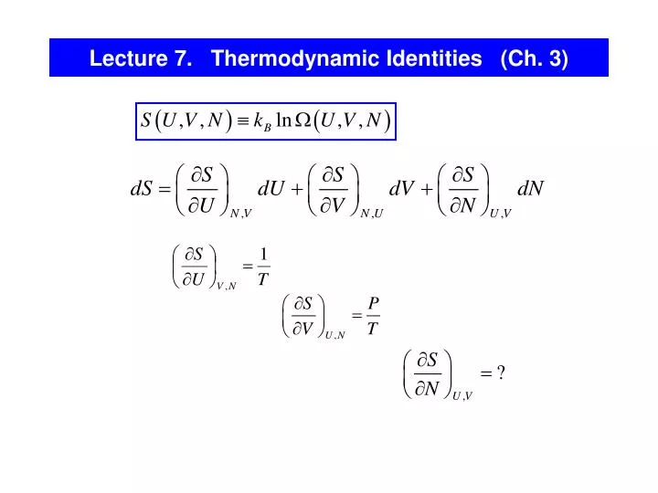
Lecture 7. Thermodynamic Identities (Ch. 3). Let’s fix V A and V B (the membrane’s position is fixed), but assume that the membrane becomes permeable for gas molecules (exchange of both U and N between the sub-systems, the molecules in A and B are the same ).

E N D
Let’s fix VA and VB (the membrane’s position is fixed),but assume that the membrane becomes permeable for gas molecules (exchange of both U and N between the sub-systems, the molecules in A and B are the same ). Diffusive Equilibrium and Chemical Potential For sub-systems in diffusive equilibrium: UA, VA, NA UB, VB, NB In equilibrium, - the chemical potential Sign “-”: out of equilibrium, the system with the larger S/N will get more particles. In other words, particles will flow from from a high /T to a low /T.
Chemical Potential: examples Einstein solid: consider a small one, with N = 3 and q = 3. let’s add one more oscillator: To keep dS = 0, we need to decrease the energy, by subtracting one energy quantum. Thus, for this system Monatomic ideal gas: At normal T and P, ln(...) > 0, and < 0 (e.g., for He, ~ - 5·10-20 J ~ - 0.3 eV. Sign “-”: usually, by adding particles to the system, we increase its entropy. To keep dS = 0, we need to subtract some energy, thus U is negative.
The Quantum Concentration n=N/V – the concentration of molecules 0 when n increases The chemical potential increases with the density of the gas or with its pressure. Thus, the molecules will flow from regions of high density to regions of lower density or from regions of high pressure to those of low pressure . when n nQ, 0 - the so-called quantum concentration (one particle per cube of side equal to the thermal de Broglie wavelength). When nQ >> n, the gas is in the classical regime. At T=300K, P=105 Pa , n << nQ. When n nQ, the quantum statistics comes into play.
Entropy Change for Different Processes The partial derivatives of S play very important roles because they determine how much the entropy is affected when U, V and N change: The last column provides the connection between statistical physics and thermodynamics.
Thermodynamic Identity for dU(S,V,N) if monotonic as a function of U (“quadratic” degrees of freedom!), may be inverted to give pressure chemical potential compare with shows how much the system’s energy changes when one particle is added to the system at fixed S and V. The chemical potential units – J. - the so-called thermodynamic identity for U This holds for quasi-static processes (T, P, are well-define throughout the system).
Thermodynamic Identities - the so-called thermodynamic identity With these abbreviations: shows how much the system’s energy changes when one particle is added to the system at fixed S and V. The chemical potential units – J. is an intensive variable, independent of the size of the system (like P, T, density). Extensive variables (U, N, S, V ...) have a magnitude proportional to the size of the system. If two identical systems are combined into one, each extensive variable is doubled in value. The thermodynamic identity holds for the quasi-static processes (T, P, are well-define throughout the system) The 1st Law for quasi-static processes (N = const): This identity holds for small changes Sprovided T and P are well defined. The coefficients may be identified as:
The Equation(s) of State for an Ideal Gas Ideal gas: (fN degrees of freedom) The “energy” equation of state (U T): The “pressure” equation of state (P T): - we have finally derived the equation of state of an ideal gas from first principles! In other words, we can calculate the thermodynamic information for an isolated system by counting all the accessible microstates as a function of N, V, and U.
Ideal Gas in a Gravitational Field Pr. 3.37. Consider a monatomic ideal gas at a height z above sea level, so each molecule has potential energy mgz in addition to its kinetic energy. Assuming that the atmosphere is isothermal (not quite right), find and re-derive the barometric equation. note that the U that appears in the Sackur-Tetrode equation represents only the kinetic energy In equilibrium, the chemical potentials between any two heights must be equal:
2 P S =const along the isentropic line 2* 1 Vf Vi V Caution: for non-quasistatic adiabatic processes, S might be non-zero!!! Pr. 3.32.A non-quasistatic compression. A cylinder with air (V = 10-3 m3, T = 300K, P =105 Pa) is compressed (very fast, non-quasistatic) by a piston (A = 0.01 m2, F = 2000N, x = 10-3m). Calculate W, Q, U, and S. An example of a non-quasistatic adiabatic process holds for all processes, energy conservation quasistatic, T and P are well-defined for any intermediate state quasistatic adiabatic isentropic Q = 0 for both non-quasistatic adiabatic The non-quasistatic process results in a higher T and a greater entropy of the final state.
Direct approach: adiabatic quasistatic isentropic adiabatic non-quasistatic
2 To calculate S, we can consider any quasistatic process that would bring the gas into the final state (S is a state function). For example, along the red line that coincides with the adiabata and then shoots straight up. Let’s neglect small variations of T along this path ( U << U, so it won’t be a big mistake to assume T const): P U = Q = 1J 1 Vf Vi V The entropy is created because it is an irreversible, non-quasistatic compression. 2 P For any quasi-static path from 1 to 2, we must have the same S. Let’s take another path – along the isotherm and then straight up: U = Q = 2J isotherm: 1 Vf Vi V “straight up”: Total gain of entropy:
The inverse process, sudden expansion of an ideal gas (2 – 3) also generates entropy (adiabatic but not quasistatic). Neither heat nor work is transferred: W = Q = 0 (we assume the whole process occurs rapidly enough so that no heat flows in through the walls). 2 P Because U is unchanged, T of the ideal gas is unchanged. The final state is identical with the state that results from a reversible isothermal expansion with the gas in thermal equilibrium with a reservoir. The work done on the gas in the reversible expansion from volume Vf to Vi: 3 1 Vf Vi V The work done on the gas is negative, the gas does positive work on the piston in an amount equal to the heat transfer into the system Thus, by going 1 2 3 , we will increase the gas entropy by