Download
1 / 16
160 likes | 276 Views
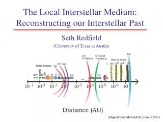
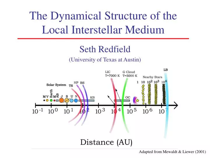
The Dynamical Structure of the Local Interstellar Medium. Seth Redfield (University of Texas at Austin). Adapted from Mewaldt & Liewer (2001). Local Bubble R ~ 100 pc; n e ~ 10 -3 cm -3 ; T ~ 10 6 K NaI spectroscopy (Lallement, Welsh, et al. 2003)

E N D
The Dynamical Structure of the Local Interstellar Medium Seth Redfield (University of Texas at Austin) Adapted from Mewaldt & Liewer (2001)
Local Bubble R ~ 100 pc; ne ~ 10-3 cm-3; T ~ 106 K NaI spectroscopy (Lallement, Welsh, et al. 2003) Soft X-rays ROSAT (Snowden et al. 1998) OVI absorption lines FUSE (Oegerle et al. 2005) OVII, OVIII emission Chandra (Smith et al. 2005) EUV emission lines CHIPS (Hurwitz et al. 2005) LISM R ~ 1-10 pc; n ~ 0.2 cm-3; T ~ 7000 K Lyman-α backscatter SOHO (Quémerais et al. 2000) He I emission Ulysses (in situ) (Witte et al. 1996) UV/Optical spectroscopy (Redfield & Linsky 2002, 2004, Welty, Hobbs, Morton 2003, Crawford 2001) Radio scintillation (Rickett et al. 2002, Bignall et al. 2006) Cold Dense Gas? R~1.4 pc; nH ~ 30 cm-3; T ~ 20 K NaI spectroscopy (Lallement, Welsh, et al. 2003) NaI + HI (Meyer et al. 2006; Heiles & Troland 2003) CO (Magnani et al. 1996) Cores (Chol Minh et al. 2003) Lallement, Welsh, et al. (2003)
Summary What are the broader implications of studying the LISM? Interaction of stars and planetary systems with their surrounding ISM environment. Heliosphere: momentum balance (v2) between solar wind and LISM. General interstellar phenomena in great detail and in three dimensions. Dynamics and Morphology: cloud-cloud interactions, collisions, shear, etc. Status of high spectral resolution LISM database. The last decade have seen a dramatic increase in the number of LISM observations. Procedure for modeling dynamical structure. Immediate implications: Sun currently located in transition material between two clouds. Compression of warm clouds to create cold clouds. Radio scintillation: connecting z~1.5 with z~10-9. Conclusions and Future Directions.
Global Kinematics Our “observables”: Centroid velocity (vR) of LISM absorption, i.e., the radial component of the projected velocity in direction (l, b) Assume the simplest dynamical structure: a single vector bulk flow. vR = v0 (cos b cos b0 cos (l0 - l) + sin b0 sin b) Questions: Can the observed LISM velocities be characterized by a rigid bulk flow, or are they chaotic? How significant are any departures (e.g., spatial correlations) from a rigid flow vector? Can multiple velocity vectors successfully characterize the majority of LISM observations?
Global Kinematics: Previous Work Lallement & Bertin (1992) Based on a small number of sightlines (~10) it was determined that in general, a single flow vector could characterize the motion of the LISM (Crutcher 1982, Lallement & Bertin 1992). Although departures from a simple single velocity flow have been detected: Separate dynamical clouds (Frisch et al. 2002) Deceleration at the leading edge of the LIC (Redfield & Linsky 2001)
Current LISM Sample 160 targets within 100 pc observed at high and moderate resolution that contain 270 LISM absorption components (~60% of UV observations taken for other purposes). The majority (77%) of observations deviate by > 3 from a single LISM vector.
Dynamical Modeling Procedure Iterative process: Fit dataset Remove outliers (in velocity and space) Repeat until satisfactory fit (use F-test to determine stopping point) Remove successful dynamical cloud sightlines from dataset Start over. Assumptions: All motions are rigid velocity vectors (i.e., a tensor dynamical characterization may result in two separate dynamical clouds, close in space, and with similar velocity vectors). The projected morphology of all clouds are contiguous (i.e., no “swiss cheese” clouds) Results: Fits largest surface area structures first (e.g., LIC and G vectors derived immediately). 15 velocity vectors satisfy 80% of LISM database. All velocity vectors are similar, and approximately opposite to the motion of the Sun. About 1/3rd of the dynamical clouds are filamentary. Distribution of clouds along boundary of the LIC and G clouds.
Upwind Velocity Distribution Relative to Sun: Upwind Velocity Distribution Relative to LSR: Vector Distribution: All LISM vectors are coming from a narrow range of directions A relatively wide range of velocity magnitudes, with mean around 20 km/s relative to LSR The solar trajectory (upstream: l ~ 208, b ~ -32, v ~ -13 km/s) is in almost the exact opposite direction (Dehnen & Binney 1998) Many dynamical clouds have filamentary structures possibly due to collisional interfaces Redfield & Linsky (2007)
The Current Solar Environment The current location of the Sun appears to be in the transition material between the LIC and the G clouds. *Möbius et al. (2004)
Leo Cold Cloud A cold (20 K) cloud has been recently determined to reside < 40 pc from the Sun by Meyer et al. (2006). In the direction of the Leo Cold Cloud, high radial velocity differences imply compression, and may point to the origin of the observed cold cloud. Macroscopic Velocity Differences near Leo Cold Cloud All V magnitudes for clouds that share the same line of sight. Indicate that macroscopic motions can induce compression and shear flows. Transonic turbulent compression by warm interstellar clouds can successfully create cold neutral clouds (Vazquez-Semadeni et al. 2006). Redfield & Linsky (2007) LIC/G
Radio Scintillation: IntraDay Variables (IDVs) 1% of all radio quasars show short timescale variability (hours). Diffraction of intervening screen can cause time delays in signal - use to get transverse motion of scintillating screen. As Earth moves through projection of diffraction pattern, the characteristic timescale of scintillation varies - which is repeatable over several years. Set characteristic scale length (~104 km) to Fresnel scale to put limits on screen distance: L < 10 pc! Dennett-Thorpe & de Bruyn (2002) Bignall et al. (2006)
Annual Scintillation Signature Annual variation of scintillation timescale is fit with 5 free parameters: diffraction scale length, axial ratio, orientation, and transverse velocity. For B1257-326, our derived transverse velocity of the Aur Cloud, which lies along the line of sight toward the quasar B1257-326, is consistent with the radio scintillation observations! Bignall et al. (2006)
Conclusions and Future Work Developed a comprehensive dynamical model of the LISM 15 rigid velocity vectors successfully characterize 80% of all LISM observations Vectors are similar and antiparallel to solar motion 1/3rd of all dynamical clouds are filamentary, indicative of interaction interfaces Clouds have distinct physical properties in addition to their kinematics Sun currently located in transition material between LIC and G clouds Highly turbulent clouds show lower depletion levels (i.e., more ions in the gas phase) Dynamical model may be able to test origin mechanisms of cold clouds Transverse LISM cloud velocities are consistent with transverse radio scintillation screen velocities Foundation to construct a fully 3D morphological and physical model 3D morphological model of LISM in order to constrain distances of absorbing material