Download
1 / 25
250 likes | 371 Views
Evolutionary Computation. Evolving Neural Network Topologies. Project Problem. There is a class of problems that are not linearly separable The XOR function is a member of this class The BACKPROPAGATION algorithm can express a variety of these non-linear decision surfaces. Project Problem.

E N D
EvolutionaryComputation Evolving Neural Network Topologies
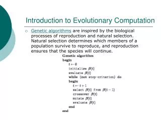
Project Problem • There is a class of problems that are not linearly separable • The XOR function is a member of this class • The BACKPROPAGATION algorithm can express a variety of these non-linear decision surfaces
Project Problem • Non-linear decision surfaces can’t be “learned” with a single perceptron • Backprop uses a multi-layer approach where there is a number of input units, a number of “hidden” units, and the corresponding output units
Parametric Optimization • Parametric Optimization was the goal of this project • The parameter to be optimized was the number of hidden units in the hidden layer of a backprop network used to learn the output for the XOR benchmark function
Tool Boxes • A neural network tool box developed by Herve Abdi (available from Matlab Central) was used for the backprop application • The Genetic Algorithm for Function Optimization (GAOT) was used for the GA application
Graphical Illustrations • The next plot shows the randomness associated with successive runs of the backprop algorithm • xx = mytestbpg(1,5000,0.25) • Where 1 is the number of hidden units, 5000 is the number of training iterations, and 0.25 is the learning rate
The error from the above plot (and the following) is calculated as follows: Graphical Illustrations
Graphical Illustrations • E(n) is the error at time epoch n • Ti(n) = [0 11 0] is the output of the target function with input sets: (0,0), (0,1), (1,0), and (1,1) at time epoch n • Oi(n) = [o1 o2 o3 o4] is the output of the backprop network at time epoch n • Notice that the training examples will cover the entire state space of this function
Graphical Illustrations • The next few plots will show the effects of the rate of error convergence for different numbers of hidden units
Parametric Optimization • The GA supplied by the GAOT tool box was used to optimize the number of hidden units needed for the XOR backprop benchmark • A real-valued (floating point representation instead of binary value representation) was used in conjunction with the selection, mutation, and cross-over operators
Parametric Optimization • The fitness (evaluation) function is the driving factor for the GA in the GAOT toolbox • The fitness function is specific to the problem at hand
Parametric Optimization • Authors of the “NEAT” paper give the following results for their NeuroEvolutionary implementation • Optimum number of hidden nodes (average value): 2.35 • Average number of generations: 32
Parametric Optimization • Results of my experimentation:’ • Optimum number of hidden units (average value): 2.9 • Convergence of this value after approximately 17 generations
Parametric Optimization • GA parameters: • Population size of 20 • Maximum number of generations: 50 • Backprop fixed parameters: 5000 training iterations; learning rate of 0.25 • Note: Approximately 20 minutes per run of the GA with these parameter values. Running on Matlab with 768MB of RAM at 2.2 GHz
Conclusion • Interesting experimental results. Also agrees with other researchers results • GA is a good tool to use for parameter optimization. However, the results depend on a good fitness function for the task at hand