Download
1 / 24
270 likes | 808 Views
Finite Impulse Response Filters. Outline. Many Roles for Filters Convolution Z -transforms Linear time-invariant systems Transfer functions Frequency responses Finite impulse response (FIR) filters Filter design with demonstration Cascading FIR filters demonstration Linear phase.

E N D
Outline • Many Roles for Filters • Convolution • Z-transforms • Linear time-invariant systems Transfer functions Frequency responses • Finite impulse response (FIR) filters Filter design with demonstration Cascading FIR filters demonstration Linear phase
Many Roles for Filters • Noise removal Signal and noise spectrally separated Example: bandpass filtering to suppress out-of-band noise • Analysis, synthesis, and compression Spectral analysis Examples: calculating power spectra (slides 14-10 and 14-11) and polyphase filter banks for pulse shaping (lecture 13) • Spectral shaping Data conversion (lectures 10 and 11) Channel equalization (slides 16-8 to 16-10) Symbol timing recovery (slides 13-17 to 13-20 and slide 16-7) Carrier frequency and phase recovery
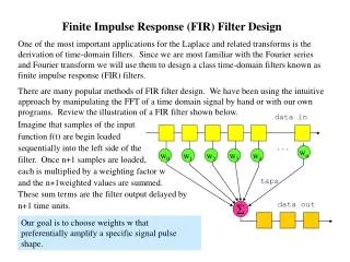
Finite Impulse Response (FIR) Filter • Same as discrete-time tapped delay line (slide 3-18) • Impulse response h[n] has finite extent n = 0,…, M-1 x[n-1] x[n] z-1 z-1 … z-1 … h[0] h[1] h[2] h[M-1] S y[n] Discrete-time convolution
h[n] Averaging filter impulse response n 0 1 2 3 Review Discrete-time Convolution Derivation • Output y[n] for inputx[n] • Any signal can be decomposedinto sum of discrete impulses • Apply linear properties • Apply shift-invariance • Apply change of variables y[n] = h[0] x[n] + h[1] x[n-1] = ( x[n] + x[n-1] ) / 2
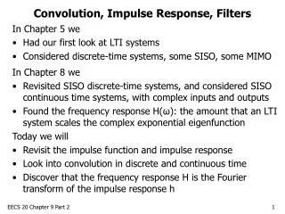
Review Convolution Comparison • Continuous-time convolution of x(t) and h(t) For each t, compute different (possibly) infinite integral • In discrete-time, replace integral with summation For each n, compute different (possibly) infinite summation • LTI system Characterized uniquely by its impulse response Its output is convolution of input and impulse response
x(t) * h(t) = y(t) 1 1 Ts t t t Ts 0 Ts 0 Ts 2Ts Convolution Demos • The Johns Hopkins University Demonstrations http://www.jhu.edu/~signals Convolution applet to animate convolution of simple signals and hand-sketched signals Convolving two rectangular pulses of same width gives triangle with width of twice the width of rectangular pulses(see Appendix E in course reader for intermediate work) What about convolving two pulses of different lengths?
Review Z-transform Definition • For discrete-time systems, z-transforms play same role as Laplace transforms do in continuous-time Inverse transform requires contour integration over closed contour (region) R Contour integration covered in a Complex Analysis course • Compute forward and inverse transforms using transform pairs and properties Bilateral Forward z-transform Bilateral Inverse z-transform
h[n] = d[n] Region of convergence: entire z-plane h[n] = d[n-1] Region of convergence: entire z-plane except z = 0 h[n-1] z-1 H(z) h[n] = an u[n] Region of convergence for summation: |z| > |a| |z| > |a| is the complement of a disk Review Three Common Z-transform Pairs Finite extent sequences Infinite extent sequence
Region of the complex z-plane for which forward z-transform converges Four possibilities (z = 0 is special case that may or may not be included) Im{z} Im{z} Entire plane Disk Re{z} Re{z} Im{z} Im{z} Intersection of a disk and complement of a disk Complement of a disk Re{z} Re{z} Review Region of Convergence
Review System Transfer Function • Z-transform of system’s impulse response Impulse response uniquely represents an LTI system • Example: FIR filter with M taps (slide 5-4) Transfer function H(z) is polynomial in powers of z-1 Region of convergence (ROC) is entire z-plane except z = 0 • Since ROC includes unit circle, substitute z = ej w into transfer function to obtain frequency response
Continuous Time Delay by T seconds Impulse response Frequency response Discrete Time Delay by 1 sample Impulse response Frequency response y(t) x(t) Example: Ideal Delay y[n] x[n] Zero Initial Conditions w = W T Allpass Filter Linear Phase
Linear Time-Invariant Systems • Fundamental Theorem of Linear Systems If a complex sinusoid were input into an LTI system, then output would be input scaled by frequency response of LTI system (evaluated at complex sinusoidal frequency) Scaling may attenuate input signal and shift it in phase Example in continuous time: see handout F Example in discrete time. Let x[n] = e j w n, H(w) is discrete-time Fourier transform of h[n]H(w) is also called the frequency response x[n] * h[n] H(w)
Frequency Response • Continuous-timeLTI system • Discrete-timeLTI system • For real-valued impulse response H(e -j ω) = H*(e j ω) Input Output
Frequency Response • System response to complex sinusoid e jwn for all possible frequencies win radians per sample: Lowpass filter: passes low and attenuates high frequencies Linear phase: must be FIR filter with impulse response that is symmetric or anti-symmetric about its midpoint • Not all FIR filters exhibit linear phase |H(w)| |H(w)| Linearphase stopband stopband w w -wstop -wp wp wstop passband
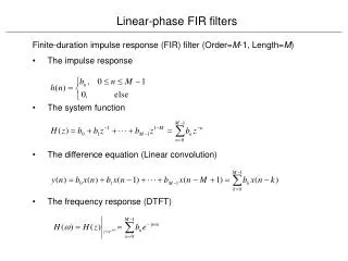
Filter Design • Specify a desired piecewise constant magnitude response • Lowpass filter example w [0, wp], mag [1-dp, 1] w [ws, p], mag [0, ds] Transition band unspecified • Symmetric FIR filter design methods Windowing Least squares Remez (Parks-McClellan) Lowpass Filter Example Desired Magnitude Response forbidden 1 1-dp forbidden Achtung! forbidden ds w wp ws p Passband Transition band Stopband Red region is forbidden dp passband rippleds stopband ripple
Input-output relationship Impulse response Frequency response h[n] Two-tap averaging filter ½ n 2 1 3 x[n-1] x[n] z-1 h[0] h[1] y[n] S Example: Two-Tap Averaging Filter Linear Phase
Input-output relationship Impulse response Frequency response Example: First-Order Difference h[n] First-order difference ½ n 2 3 - ½ Generalized Linear Phase
h[n] First-order difference impulse response 1 n 3 2 -1 Cascading FIR Filters Demo • Five-tap discrete-time averaging FIR filter with input x[n] and output y[n] Standard averaging filtering scaled by 5 Lowpass filter (smooth/blur input signal) Impulse response is {1, 1, 1, 1, 1} • First-order difference FIR filter Highpass filter (sharpensinput signal) Impulse response is {1, -1}
Cascading FIR Filters Demo • DSP First, Ch. 6, Freq. Response of FIR Filters http://www.ece.gatech.edu/research/DSP/DSPFirstCD/visible/chapters/6firfreq/demos/blockd/index.htm For username/password help • From lowpass filter to highpass filter original image blurred image sharpened/blurred image • From highpass to lowpass filter original image sharpened image blurred/sharpened image • Frequencies that are zeroed out can never be recovered (e.g. DC is zeroed out by highpass filter) • Order of two LTI systems in cascade can be switched under the assumption that computations are performed in exact precision
Cascading FIR Filters Demo • Input image is 256 x 256 matrix Each pixel represented by eight-bit number in [0, 255] 0 is black and 255 is white for monitor display • Each filter applied along row then column Averaging filter adds five numbers to create output pixel Difference filter subtracts two numbers to create output pixel • Full output precision is 16 bits per pixel Demonstration uses double-precision floating-point data and arithmetic (53 bits of mantissa + sign; 11 bits for exponent) No output precision was harmed in the making of this demo
Speech signals Use phase differences in arrival to locate speaker Once speaker is located, ears are relatively insensitive to phase distortion in speech from that speaker Used in speech compression in cell phones) Linear phase crucial Audio Images Communication systems Linear phase response Need FIR filters Realizable IIR filters cannot achieve linear phase response over all frequencies Importance of Linear Phase d = ct
Importance of Linear Phase code • For images, vital visual information in phase • Original image is from Matlab Take FFT of image Set phase to zero Take inverse FFT Take FFT of image Set magnitude to one Take inverse FFT Keep imaginary part Take FFT of image Set magnitude to one Take inverse FFT Keep real part http://users.ece.utexas.edu/~bevans/courses/rtdsp/lectures/05_FIR_Filters/Original%20Image.tif
Finite Impulse Response Filters • Duration of impulse response h[n] is finite, i.e. zero-valued for noutside interval [0, M-1]: Output depends on current input and previous M-1 inputs Summation to compute y[k] reduces to a vector dot product between M input samples in the vector and M values of the impulse response in vector • What instruction set architecture features would you add to accelerate FIR filtering?