Download
1 / 30
330 likes | 391 Views
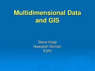
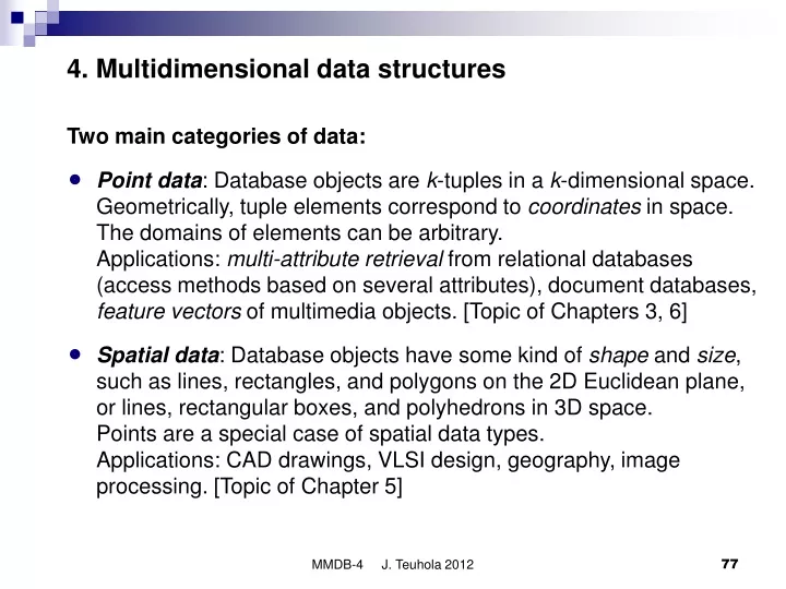
4. Multidimensional data structures. Two main categories of data:

E N D
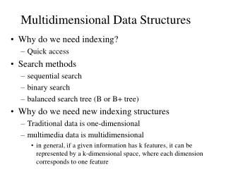
4. Multidimensional data structures Two main categories of data: • Point data: Database objects are k-tuples in a k-dimensional space.Geometrically, tuple elements correspond to coordinates in space. The domains of elements can be arbitrary.Applications: multi-attribute retrieval from relational databases(access methods based on several attributes), document databases,feature vectors of multimedia objects. [Topic of Chapters 3, 6] • Spatial data: Database objects have some kind of shape and size, such as lines, rectangles, and polygons on the 2D Euclidean plane,or lines, rectangular boxes, and polyhedrons in 3D space.Points are a special case of spatial data types.Applications: CAD drawings, VLSI design, geography, imageprocessing. [Topic of Chapter 5] MMDB-4 J. Teuhola 2012
Multidimensional data structures: preliminaries Terminology: • PAM = Point Access Method • SAM = Spatial Access Method General requirements for multidimensional data structures: • Good storage utilization should be guaranteed (70% is sufficient) • Simple tasks should require only a small number of disk accesses • Different dimensions should be treated in a symmetric way • Clustering of objects should conform with geometric proximity, to support efficient processing of range queries. • The structure should enable dynamic reorganization, when the dataset grows and shrinks (such as B-tree, linear hashing, etc.). • Algorithms for search and update should be simple. • The structure should support different kinds of queries. MMDB-4 J. Teuhola 2012
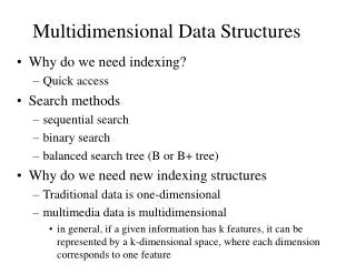
Illustration of basic query types in 2 dimensions dim1 1 2 3 4 5 6 7 8 9 10 11 12 13 14 15 X = datapoint A B C D E F G H I J K L M N X X X X X X Rangesearch:(10..13, D..G) X dim2 X X X X X Exact match: (8,J) Partial match: (4,*) MMDB-4 J. Teuhola 2012
Typical properties of multidimensional indexesin external memory • Tree structure, with disk pages as nodes • Internal nodes (directory) contain branching info + child pointers • Leaf nodes contain actual data points (vectors) • Points should be clustered so that spatially adjacent points are positioned in the same leaf nodes. • Page overflow is handled by a split, plus maintenance of the parent; the overflow may propagate upwards. • Page underflow is handled by merging siblings, plus maintaining the parent data; the underflow may propagate upwards. • GiST = Generalized Search Tree (Hellerstein, Naughton, Pfeffer; 1995): Generic tree supporting of the above principles • GiST implementation in Informix Server (Kornacker 1999) MMDB-4 J. Teuhola 2012
Arranging a multidimensional point space • Fixed number (k) of dimensions, each with its own domain of values. • Variable-dimensional objects (such as documents with keywords) may be mapped to a fixed-length representation (e.g. signature, bitmap, etc.) • Typical approach for arranging points:Repeated partitioning of the point set into a hierarchy: • space-driven:Partition the current space intotwo/four/… equal-sized halves,and split the point set accordingly, • data-driven:Partition the point set into two ormore subsets in a balanced way. MMDB-4 J. Teuhola 2012
Example of space-driven partitioning: Quadtree Root NW SE SW NE . . . . . . . . . . . . . . . .Data points in leaf nodes Demo on Quadtree (plus some other structures): http://www.cs.umd.edu/~brabec/quadtree/ MMDB-4 J. Teuhola 2012
Multidimensional query types • Exact-match queries: All coordinates (attributes) are fixed in the query. Logarithmic complexity should be achieved. • Partial-match queries: Only t out of total k coordinates are specifiedin the query. The rest may have arbitrary values.Lower bound for worst-case complexity: (n1-t/k). • Range queries: For each dimension, a range of values is specified. Exact match: range = [c,c], partial-match: (-, ) for some coordinate. • Best-match queries: Find the nearest neighbor of point/area, specified by the query conditions (exact or range). • Finding k nearest neighbors: Generalization of the above. • Ranking query: k nearest neighbors in the order of proximity. MMDB-4 J. Teuhola 2012
Literature on multidimensional data structures • Gaede, V., Günther, O.:”Multidimensional Access Methods”, ACM Computing Surveys, Vol. 30, No. 2, 1998, pp. 170-231. • Böhm, C., Berchtold, S., Kriegel, H.-P., Michel, U.:”Multidimensional Index Structures in Relational Databases”,Journal of Intelligent Information Systems, Vol. 15, 2000,pp. 51-70. • Böhm, C., Berchtold, S., Keim, D.A.: ”Searching in High-Dimensional Spaces – Index Structures for Improving the Performance of Multimedia Databases”, ACM Computing Surveys, Vol. 33, No. 3, 2001, pp. 322-373. MMDB-4 J. Teuhola 2012
Mapping to one dimension: Z-order • First idea: make a concatenation of coordinate values, and builda 1-dimensional B+-tree index on the combined values.Problem: Supports well the ‘leftmost’ dimensions but not others. • More symmetric solution:Shuffle (= interleave) the binary representations of coordinates. Denote - number of dimensions = k - range of coordinate values = 0..2d-1. - arbitrary point P = <P0, ..., Pk-1>, or in binary form: <<P00, P01,..., P0,d-1>, < P10, P11,..., P1,d-1>,..., Pk-1,0, Pk,1,..., Pk-1,d-1 >> - shuffled binary representation: < P00, P10, ..., Pk-1,0, P01, P11, ..., Pk-1,1, ..., P0,d-1, P1,d-1, ..., Pk-1,d-1> • Z-order: If P and Q are points in k-dimensional space, then P Z Q if and only if shuffle(P) shuffle(Q) • Data structure: Normal 1-dimensional B+-tree, storing shuffled representations of points. MMDB-4 J. Teuhola 2012
7 6 5 4 3 2 1 0 0 1 2 3 4 5 6 7 Example of z-order on a 2D plane (k=2, d=3) MMDB-4 J. Teuhola 2012
Z-order features Background: • Z-order defines a space-filling curve, where most jumps are local. Generalizations: • Different merging orders can be defined for domains that are not equal-sized.Bit mapping tables are then needed for shuffle and unshuffle. Operations on the z-order structure: • Exact match, insert, delete and modify are simple (one-dimensional) B+-tree operations (using the shuffled key). • More demanding: Range search MMDB-4 J. Teuhola 2012
Range search from z-order • Generate k-dimensional search regions (SR), by repeated partitioning of the whole space. • The set of satisfying points is the query region (QR). • The idea is to cover QR with one or more SRs. • Both QR and SR are k-dimensional (hyper-)rectangles. • During partitioning, a new SR may lie in three positions withrespect to QR: (1) SR is outside QR; SR contains no points that would satisfy the query. SR can be discarded. (2) SR is inside QR; all points in SR satisfy the query. The related tuples are retrieved, unshuffled, and returned to the caller. (3) SR and QR overlap; SR is split into two smaller SRs, which are handled recursively. MMDB-4 J. Teuhola 2012
Notes on range search from z-ordered points • Testing the positions of SR and QR with respect to each other does not require access to the data. • For efficiency, we should aim at subregions, which constitute a contiguous subsequence of the z-order. Rule: On the i’th level of recursion, split SR evenly into two SRs along dimension (i mod k). Notation for a region: • lower:upper ranges for k dimensions: <l0:u0, ..., lk-1:uk-1>. • Splitting the SR on the i’th attribute means that we get two SRs: SRleft = left(SR, i) = <l0:u0, ..., li : (li+ui-1)/2, ..., lk-1:uk-1> SRright = right(SR, i) = <l0:u0, ..., (li+ui+1)/2 : ui, ..., lk-1:uk-1> MMDB-4 J. Teuhola 2012
Range search algorithm for z-order RangeSearch(QR, SR, level) -- Initially SR is the whole k-dimensional domain space, and level = 0. if SR QR is empty then do nothing elseif SR QR then SRlo := <l0, ..., lk-1> of SR -- bottom-left corner SRhi := <u0, ..., uk-1> of SR -- top-right corner read tuple twhere key shuffle(SRlo) whilet shuffle(SRhi) do report unshuffle(t) read the next t -- in z-order else RangeSearch(QR, left(SR, attr[level mod k]), level+1) RangeSearch(QR, right(SR, attr[level mod k]), level+1) end MMDB-4 J. Teuhola 2012
7 6 5 4 3 2 1 0 0 1 2 3 4 5 6 7 Example range search from z-order • k = 2, d = 3, QR = <1:3, 0:4> • Points: {(0,3), (1, 4), (2,1), (2,3), (2,6), (4,7), (6,2), (6,5), (7,5)} Note: The thick lines enclose the successful SRs; the actual bounds for the SR-intervals are integer-valued. MMDB-4 J. Teuhola 2012
<0:7, 0:7> <4:7, 0:7> (outside) <0:3, 0:7> <0:3, 4:7> <0:3, 0:3> <0:1, 0:3> <2:3, 0:3> (inside) <0:1, 4:7> <2:3, 4:7> <0:1, 0:1> <0:1, 2:3> <0:1, 4:5> <0:1, 6:7> (outside) <2:3, 4:5> <2:3, 6:7> (outside) <0:0, 0:1> (outside) <0:0, 2:3> (outside) <0:0, 4:5> (outside) <2:2, 4:5> <3:3, 4:5> <1:1, 0:1> (inside) <1:1, 2:3> (inside) <1:1, 4:5> <2:2, 4:4> (inside) <3:3, 4:4> (inside) <1:1, 4:4> (inside) <1:1, 4:5> (outside) <2:2, 5:5> (outside) <3:3, 5:5> (outside) Development of SRs in the range search <1:3, 0:4> MMDB-4 J. Teuhola 2012
Observations from z-order range search • The points within each SR are consecutive in z-order, and therefore accessible sequentially, starting e.g. from the bottom-left corner of the block. • On the border of QR, a number of small SRs are created.Most of them do not cause a page fault, because they are close in z-order. However, internal processing may be considerable. • The recursion stack can be compressed to 2 tuple length in bitsbased on the fact that higher-level SRs may be deduced froma given SR). • Possible modification: Inspect a superset of QR, by stopping at a level that is suitable for effective disk processing. Generalizations: • Universal B-tree (UB-tree): Variable-depth representation • Pyramid tree: Optimized for range queries from high-dim. data • The idea can be extended also to spatial objects. MMDB-4 J. Teuhola 2012
kd-tree • k-dimensional tree, but structurally binary • Balanced partitioning of the point set (not the space) • Recursive splitting according to a single dimension at a time • Splitting dimension is varied in a cyclic manner • Originally a main-memory structure • Not dynamic maintenance of balance (only in building) Building a kd-tree from a given point set: 1. Find the median of the first dimension. 2. Split the point set into two subsets by using the median as a discriminator value. 3. Store the discriminator in the root 4. Build subtrees recursively, but using different dimensions in cyclic order when determining the discriminator. Complexity: O(kN log N) for N points. MMDB-4 J. Teuhola 2012
Versions of kd-tree(compare with B-tree vs. B+-tree) • Homogeneous:Discriminator points are stored in internal nodes • Non-homogeneous:Discriminator values are stored in internal nodes, but all points (including the discriminator points) are stored in the leaves. Example: Non-homogeneous kd-tree. x2 x>2 y3 y>3 y2 y>2 x1 x>1 x1 x>1 x3 x>3 x4 x>4 (1,2) (2,3) (1,5) (2,4) (3,1) (4,2) (4,4) (5,3) 5 4 3 y 2 1 1 2 3 4 5 x MMDB-4 J. Teuhola 2012
Searching from a (non-homogeneous) kd-tree (a) Exact-match query: • Follow a path down from the root: On the i’th level compare the(i mod k)’th coordinate c with the discriminator d of the node. • If c d then go to the left subtree, otherwise to the right. • Continue to the leaf. If all coordinates match, return the point. Balanced kd-trees: search cost O(log N)Randomly built kd-trees: expected search cost O(log N) (b) Partial-match query: • If the i’th dimension is not specified in the query, we must search both subtrees on levels j where (j mod k) = i. • Otherwise, branch as in (a). If t (<k) out of k dimensions are fixed, then the cost isapproximately O(t N1-t/k). MMDB-4 J. Teuhola 2012
Searching from a (non-homogeneous) kd-tree (cont.) (c) Range query: • On the i’th level, if the query range of coordinate (i mod k) istotally below the discriminator d, then go to the left subtree;if it is totally above d, then go to the right. • Otherwise both subtrees must be searched. Worst-case complexity: O(N1-1/k + F), where F is the result size. Average-case complexity: O(log N + F). MMDB-4 J. Teuhola 2012
Updating the kd-tree Insert and delete: • Generalize the normal binary search tree operations correspondingly. • But: The balance is not maintained dynamically. • The shape of the tree depends on the insertion order • Reorganization may be needed from time to time. • Balanced kd-trees exist, but complicated Demo on kd-tree (plus some other structures): • http://www.cs.umd.edu/~brabec/quadtree/ MMDB-4 J. Teuhola 2012
Adapting the kd-tree to external memory: sketch • Group neighboring leaves into data pages. • Group neighboring internal nodes into index pages. • Dynamic management of pages should be solved. MMDB-4 J. Teuhola 2012
Adapting the kd-tree to external memory: kd-B-tree • kd-B-tree was one of the first (1981) multidimensional structurestailored to external memory; more sophisticated tree structureswere developed later. • Structure:Multiway tree consisting of two kinds of nodes: (1) Region pages: - Internal nodes that comprise the actual index (directory) - A region is a rectangular block in k-dimensional space - A region page represents the partition of the block into subregions. - Splitting into subregions is done similar to the k-d-tree. (2) Point pages: - Leaf nodes that contain actual points (k coordinate values per point) MMDB-4 J. Teuhola 2012
Schematic exampleof a kd-B-tree: MMDB-4 J. Teuhola 2012
Searching from a kd-B-tree • Exact-match queries: • Start from the root page. • Within the page-related local kd-tree, branch repeatedlyto the correct region. • Follow the child pointer related to the obtained region • Repeat branching in the subtree contained in the child page • When reaching a leaf, check the point matches • Partial-match and range queries: • As above, but branch to all sub-regions intersectingthe query region. MMDB-4 J. Teuhola 2012
Inserting a new point in a kd-B-tree • Insert the point into the correct leaf page, if it fits • If a leaf overflows, it is split according to the ‘next’ dimension,using the median value as the discriminator.The split information is propagated to the parent page. • If the parent overflows, it is split into two. A new split plane is chosen to separate the sub-regions of the new pages. • A sub-region may appear in three positions: • Left to the cut plane: Move the sub-region to the ‘left’ page. • Right to the cut plane: Move the sub-region to the ‘right’ page. • The plane cuts the sub-region:Split the sub-region into left and right halves, and propagate the split to the corresponding child node. • Overflow may propagate up and down;not quite ‘incremental’ update. MMDB-4 J. Teuhola 2012
Deletion of a point from a kd-B-tree • First search, then delete • Underflow: Page utilization drops below a threshold.Problem: A region can be merged only with its buddy, and the buddy region may have been partitioned into subregions and spread over multiple pages.Solution: This part of the tree must be rebuilt. • Thus, deletion is not quite ‘incremental’, either. • Storage utilization of kd-B-tree: Observed value about 60% 10% (decent). MMDB-4 J. Teuhola 2012
Other multidimensional indexes for point data LSD-tree • Adaptation of kd-tree; part of the index kept in the main memory R-tree ( Rectangle tree) • Based on a hierarchy of bounding boxes. • Developed for spatial objects, used often for low-dim. points, too. TV-tree (Telescope Vector tree) • Nodes have a small varying set of active dimensions, which are used in distance calculations. M-tree • Index for points in a metric space: A distance function satisfies:(1) symmetry, (2) positivity, and (3) triangle inequality • Developed especially for MMDBs: distance of objects based on multimedia features (shape, texture, color, patterns, sound, …) MMDB-4 J. Teuhola 2012
‘Curse of dimensionality’ • General problem of high-dimensional spaces • Non-intuitive effects:, e.g. the volume grows exponentially with the #dimensions • Index regions tend to be highly overlapping • Neighboring objects tend to share a large part of the coordinate values. • Assuming uniformity of point distribution will lead to very ineffective indexing. • Think of a 100-dimensional kd-tree: A balanced tree supporting one splitpoint per dimension has 100 levels and 2100 leaves! • In the index, one should choose the coordinates, which arethe best discriminators between subsets. MMDB-4 J. Teuhola 2012